20+ Excel Table tricks to turbo charge your data

Excel Table Trick # 3. Structured references

My personal favourite feature of tables and beyond doubt it is one big advancement. For example you want to calculate the average per unit profit on the sales made so far.

To do it as per normal way follow these steps:

Step 1: Open tab named SR3 and in cell E4 put the following formula to calculate total revenue generated:

=C4*D4

Step 2: Drag the fill handler to paste the apply similar formula to next cells. Remember as cell reference is relative so it will auto update as you drag it to next rows. Doing it successfully will give you total revenue.

Step 3: In cell G4 put this formula to calculate profit margin:

=(E4-F4)/E4*100

Step 4: Executing the third step will give you profit margin in decimals. To round it up to 0 decimal place replace the formula in G4 with this:

=ROUND((E4-F4)/E4*100,0)

We have simply enclosed the whole calculation inside round function to round the figure to integer i.e. zero decimal place. Drag the fill handler to populate rest of the cells or simply double click it.

To do it using structured references follow these steps:

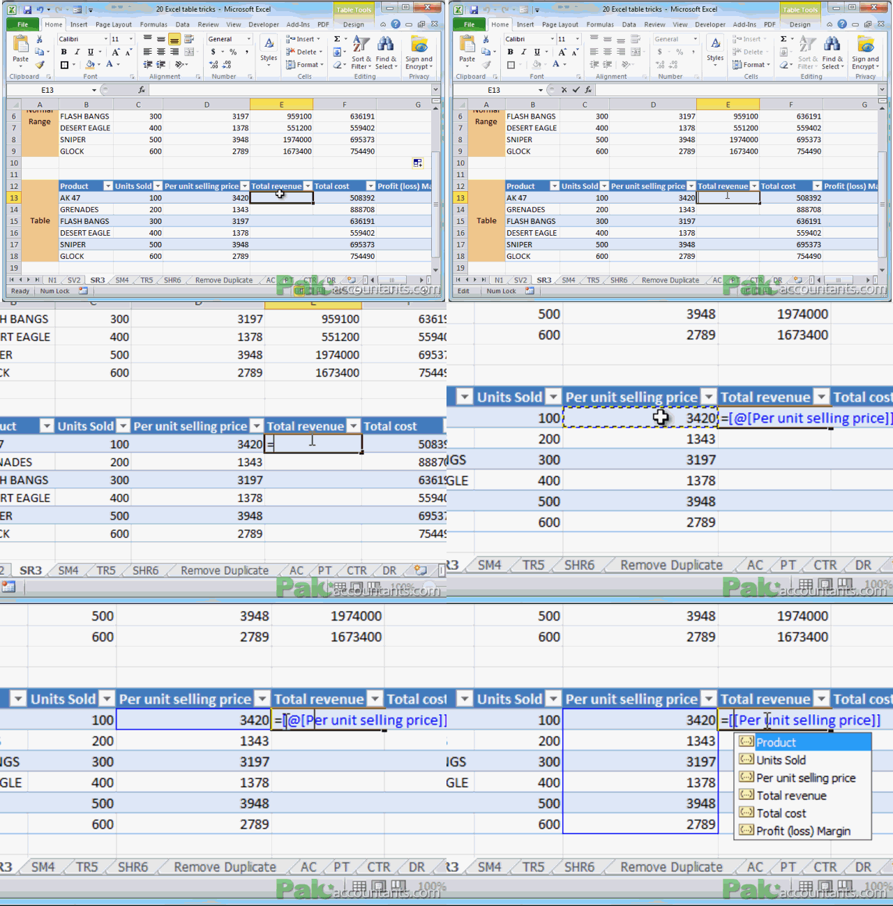
Step 1: having SR3 tab still active scroll down to cell E13 press F2 to enter edit mode and hit “=” key on the keyboard. Click on cell D13 and you will notice that formula will look like this: =[@[Per unit selling price]]

Instead of having =D13 why are we getting it? well this is called structured reference system which is part of table feature in Excel. It uses table name and column names to identify the data for function to operate instead of cell references. [Per unit selling price] is an address in itself. Remember to represent table columns excel uses square brackets [ ]. @ sign means “at this row” that means it will not consider the whole per unit selling price column. If we remove @ sign you will observe that active area expands to whole column. Consider following animation to understand this phenomena:

Back to our calculation.

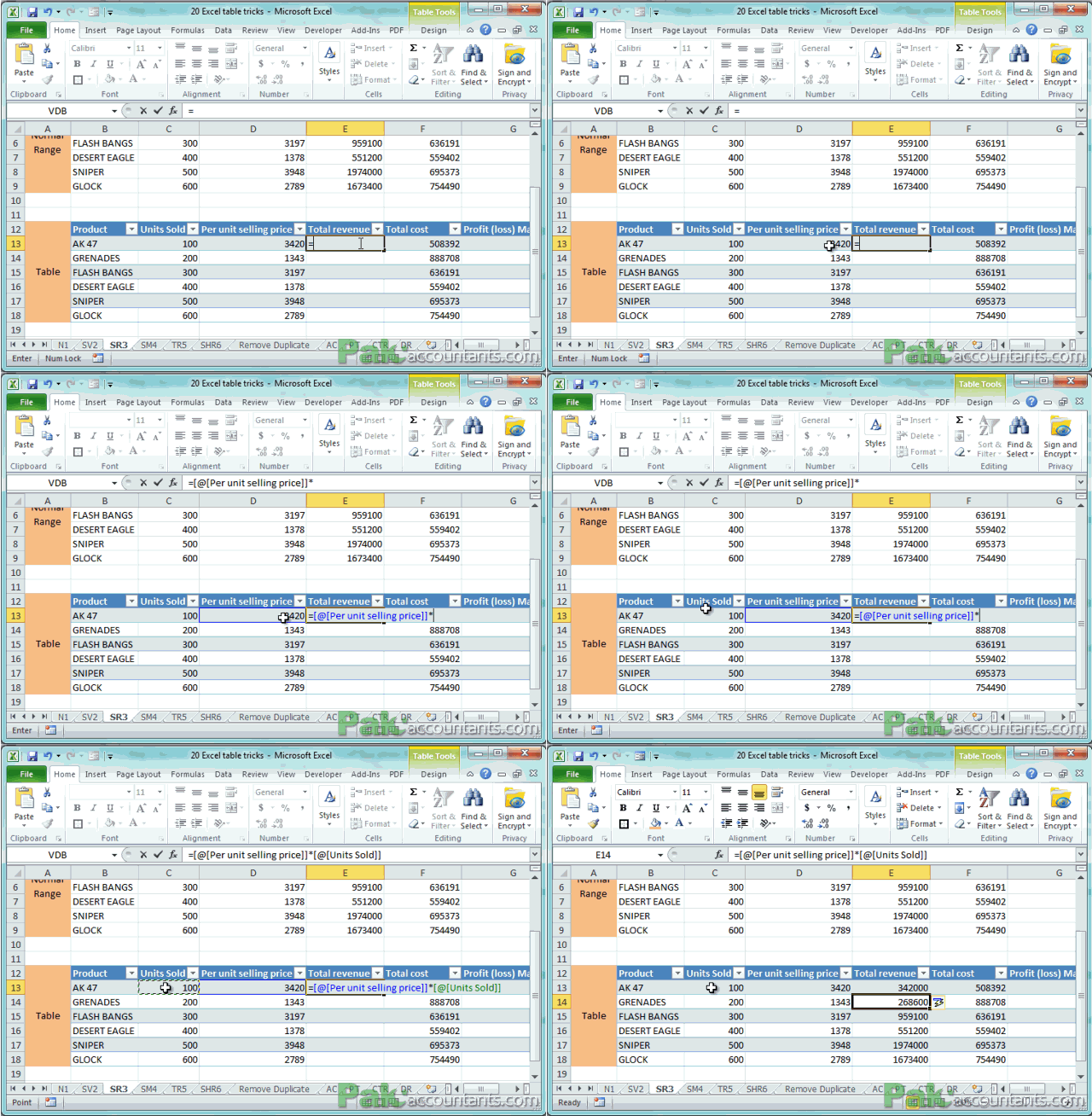
Step 2: Make sure you have done step 1 until you get: =[@[Per unit selling price]]. Hit “*” asterisk key on the keyboard and click cell C13. Press Enter. It will give you total sales revenue figure. The moment you hit Enter the whole column will be done for you automatically. This is called calculated column feature of Excel. It will be explained further below. Watch the following video to correctly execute this step:

Step 3: Go to cell G13. Press F2 to enter edit mode. Press equals button on the keyboard. Start writing ROUND, just when you will be typing a helper list will appear and instead of writing ROUND completely use directional keys to select the function from the list and hit TAB key to insert the function in the cell. Do not press Enter to insert function as Enter key completes input.

Step 2: Once you have =ROUND( in cell G13 and still in edit mode, punch in Shift+9 to put “(” open bracket.

Step 3: Click cell E13 press minus or dash button on keyboard and click F13. Hit Shift+0 to put close bracket.

Step 4: Press “/” key on the keyboard to put hash or divide by sign and click cell E13 again.

Step 5: Put asterisk and punch in 100. Hit comma to jump to second ROUND formula’s requirement field and type 0 i.e. zero. Press Shift+0 again to close the formula and hit Enter key.

Consider following animation to execute these steps properly

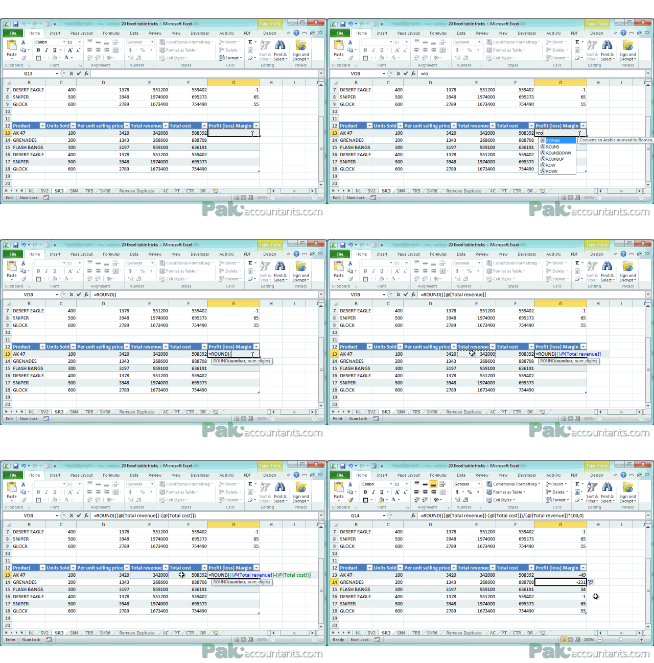
You will get the same profit percentage results as you get in normal range. But look at the formula. That is completely different makes much more sense. As you can understand what is being multiplied and what is being divided by whom. This goes hand in hand with your theoretical knowledge of calculating profit margin as well.

A detailed article on structured references and how to use it will be available soon 🙂