Multiple Column Data Validation Lists in Excel – How To

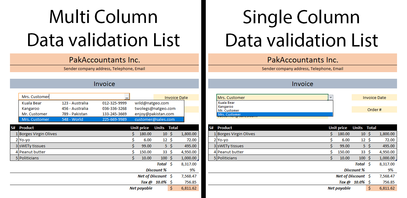
Today we are learning how to make dynamic multi columnar data validation lists in Excel that helps display much more data in the drop down list and are far superior and flexible than usual data validated lists. Here is what we will achieve by the end of this tutorial (left) and what we usually get with usual data validation lists (right)

A simple data validation list helps us display specific data range in the form of drop-down list in a desired cell.

A while back we learnt how to make dynamic data validation lists based on Excel tables that grow as the base data grow. It is much easier approach to data validation lists without the hassles of using OFFSET function coupled with unnecessary bits with more limitations still. And I implemented the same idea in designing Invoice template. However, it had single column data list and today we will be updating the same template with multi-column data validation list.

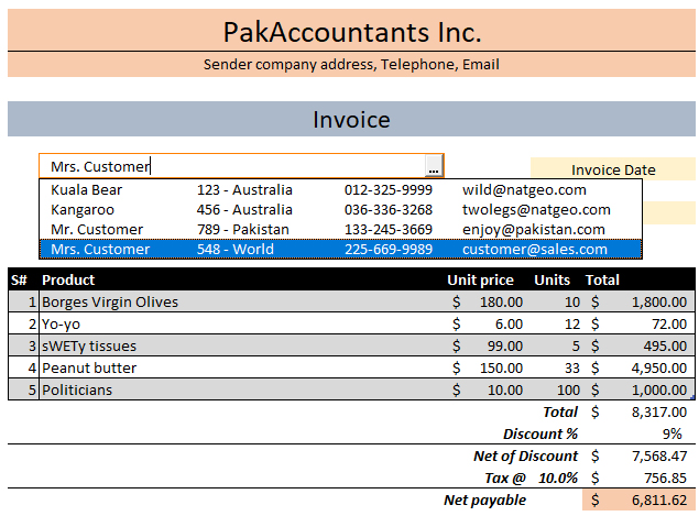
And this will be our final result once again:

Multi Column Data validation List – Step by step

Step 1: Download the excel workbook that if you intend to work along and open it in Excel.

In this workbook we already have the dummy data for customers and products. And few other techniques applied for invoice to work flawlessly. For the purpose of this tutorial I have simply removed the simple data validation list that we will update with a better solution.

To learn how this template was originally made and different techniques applied check this tutorial: FREE Excel Invoice Template V1.0 with Customer and Product list – Unlocked + Download ready!

Step 2: Go to customers worksheet and name the cell B1 CustomerName by typing it in the name box and pressing enter.

Step 3: Have an active cell inside the table in Customers worksheet and go to design tab > change the name to CustomersTable.

Step 4: Go to Formulas tab > in defined names group click Name manager > click Define Name. A new dialogue box will appear. Make the changes as following:

1. Name: CusTab
2. Refers to: =CustomersTable (same name that we gave to table in Step 3 above)

Step 5: Go to formula tab again > click define name and make the following input:

Name: CusTabFix
Refers to: =CusTab

Step 6: If you don’t already have the developer tab enabled then follow the steps as shown following:

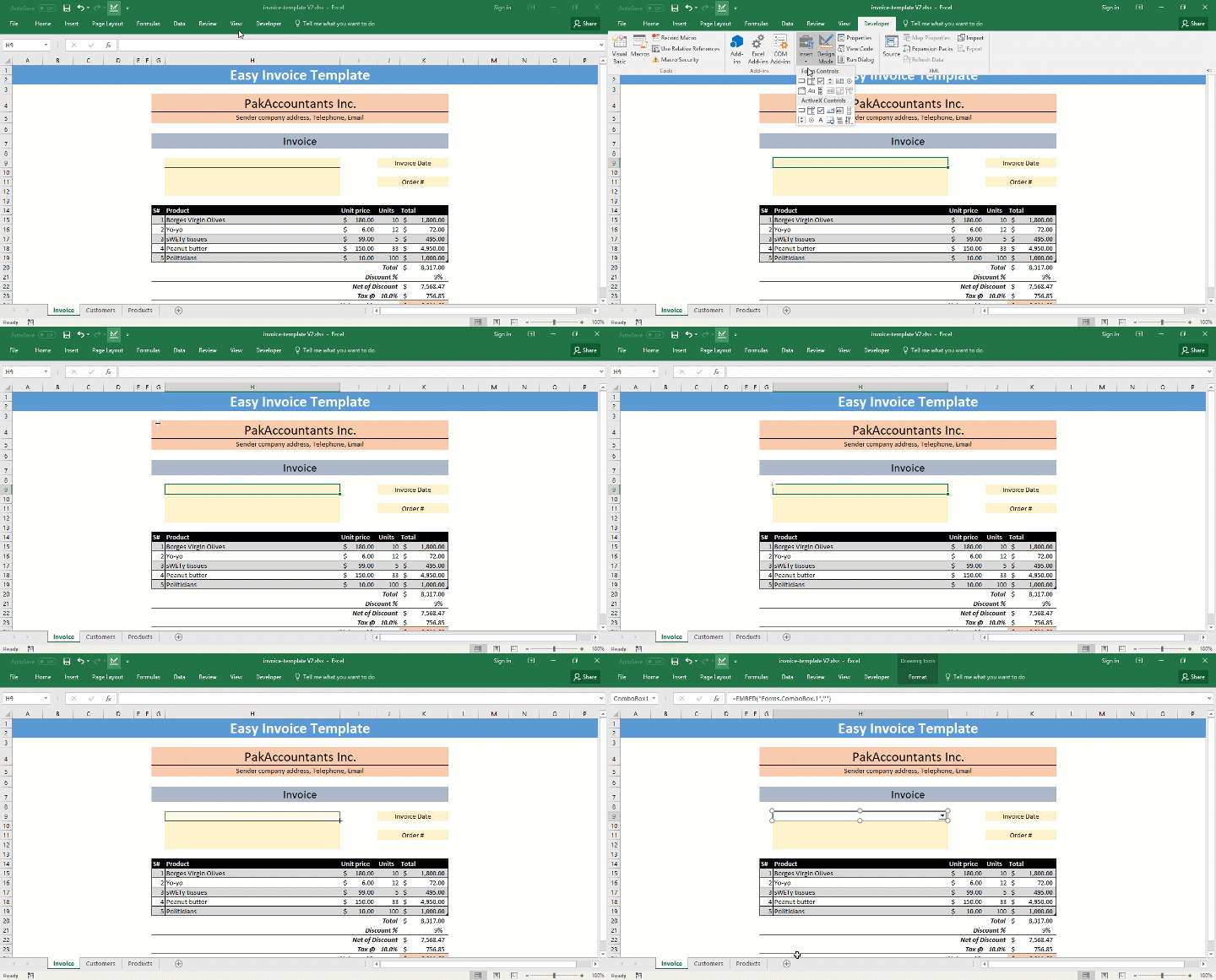
Step 4: Go to developer tab > In controls group click Insert drop down button > click combo box under active X control. Cursor will change to let you draw the combo box. Point to the cell where you want it and draw it by clicking and holding left mouse button and releasing it once done:

Step 5: Right click on inserted combo box and click properties. A long dialogue box will open with lots of properties.

Step 6: Few of the important changes that I made in properties:

1. Name: CustomersList
2. Border color: Menu bar or Orange
3. Border style: 0
4. ColumnCount: 4
5. ColumnWidths: 100 pt;80 pt;80 pt;100 pt [defines how wide each column should be in the list]
6. Drop button style: 2
7. Linked cell: CustomerName
8. ListFillRange: CusTabFix
9. ListWidth: 390 pt

This is how properties look after the changes:

And this is how it performed after the changes:

Step 7: Now that we have the list working, we can fetch the contact details of customers in the box under combo box using a formula in cell H10 of Invoice worksheet:

=IFERROR(VLOOKUP(CustomerName,CustomersTable,5,FALSE),””)

Remember CustomerName is the name we gave to cell above customer table. This cell is also used as linked cell in combo box properties and it is where we get the output of combo box. And it changes if we select a different name from the list.

Awesome!

Hope you have a good use of this technique in your work as it adds much more understanding to the user while making selections from the list.