Making Aging Analysis Reports Using Excel – How To

Hasaan Fazal

Aging analysis is helping accountants since ages and is one of those reports that are prepared mostly in Excel to track both receivables and payables. So today we are learning how to conduct aging analysis in Excel. Before we learn how to create aging reports in excel, if you want to learn more about aging or ageing analysis concept do read my explanation: What is age, aged, ageing or aging analysis?

Love reading about Excel? Subscribe my youtube channel dedicated to Excel.

Table of Contents

[vc_btn title=”Subscribe” style=”custom” custom_background=”#ff0000″ custom_text=”#ffffff” size=”lg” align=”right” i_icon_fontawesome=”fa fa-youtube-play” add_icon=”true” link=”url:https%3A%2F%2Fgoo.gl%2Fx16inH||target:%20_blank|”]

If you are new to this analysis tool and don’t know what it does I strongly recommend reading the above mentioned explanation as only then you will grab the concept of what we are going to do and why we are going to do.

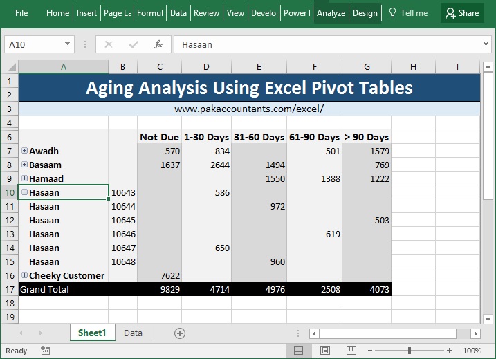
This is what our end result at the end of this tutorial looks like:

Download Fully Worked Excel file

You can download the fully worked file free of cost but if you like the effort and gained something valuable then you can set the price whatever you deem fit and pay. If you want to download it for free then simply set the price to “0”. Enjoy!

Download Now

In very few words and if I try to define aging analysis in context of receivables or debtors, then it is an analysis that helps me determine when certain sales invoices are falling due. And more importantly since how long a certain receivables are outstanding. First aspect helps me determine expected cash flows. Second helps me determine where recovery department must concentrate its efforts.

Excel Tutorial Workbook

Download this example workbook that provides you with the necessary data and to apply the concepts learnt in this tutorial

A dash at the data and requirements

Open up the workbook you downloaded and its a fairly simple data consisting of four very fragrant debtors. Each has several invoices against its name with different due dates. We want to classify invoices as follows:

Not due: The invoices which that has not fallen due yet
0-30 days: The invoices that are past due for days between 1 to 30 days.
31-60 days: The invoices that are past due for days between 31 to 60 days
61-90 days: The invoices that are past due for days between 61 to 90 days
>90 days: the invoices that are past due for more than 90 days.

Understanding the approach – Aging Analysis Reports in Excel

So it seems simple and it is simple if you know how to go about IF function and how to make multiple IF statements using AND function. Its all part of today’s discussion.

But as I always like to raise the bar a little higher than requirement so I will going one step further and will do:

aging analysis using the slabs give above i.e. not due, 0-30, 31-60 etc.
compute the number of days since the invoice is outstanding

So lets get started!

Watch a walkthrough OR continue reading for something additional!

You can either watch the following video on aging analysis in Excel to prepare basic aging analysis report OR continue reading to learn additional techniques involving conditional formatting and sparklines!

[arve url=”https://youtu.be/E0-u1Tz1JCY”/]

Adding column headers

We need to add few headings here to accommodate our requirement. So in cell

E1 type: Days outstanding
F1 type: Not due
G1 type: 0-30 days
H1 type: 31-60 days
I1 type: 61-90 days
J1 type: >90 days

Giving Data Wings Meaning! – Number crunching Time!

Step 1: In cell E5 put the following formula press Enter:

=IF(TODAY()>C5,TODAY()-C5,0)

This formula checks that if today’s date is later or greater than the date mentioned in cell C5 the deduct today’s date from the date in cell C2 to calculate the number of days. However, if today’s date is earlier than the date in C5 then put 0 as a result.

Step 2: To apply the same formula in order to calculate the days for all the invoices simple double click the fill handler and it will populate the cells immediately of column E.

Giving Data even more meaning!

Although we have calculated number of days and manager can easily sort and filter the column to find the invoices exceeding certain number of days. But using conditional formatting feature in Excel we can create a sort of heatmap to show values with long outstanding period as red and the ones that are in favourable time range as blue or similar color. By adding colors to the data, its much easier to identify and focus on important aspects of data. Follow these steps to accomplish it

Step 1: Select the values in Column E that you just calculated using formula. You can make selection with mouse or using keyboard shortcuts. To learn how to select using shortcuts read this: 40+ Excel navigational shortcuts to make accounting job super efficient

Step 2: Go to Home tab > Styles group > click the conditional formatting drop down > click new rule. A new dialogue box will appear

Step 3: Make sure the first option is selected. From the format style drop down selection menu select 3-color scale. This will enable three shades possibility.

Step 4: From type drop-down menu select number option under each of the three categories i.e. minimum, midpoint and maximum.

Step 5: Set the values as following:

minimum: 0
midpoint: 60
maximum: 90

Step 6: Select the colors you like for minimum, midpoint and maximum values. I chose blue for minimum, beige for midpoint and red for maximum. You can select any that suits your need and liking. Click OK

Joys!!! now you can instantly see what invoice needs immediate attention. (It seems this company’s recovery department is doing nothing at all!!!)

Aging Analysis Report in Excel! – Finding the lazy ones!

Now the next part which is our actual requirement i.e. to have the ageing or aging or aged analysis of each of the invoices. Follow along:

Step 1: In cell F5 put the following formula:

=IF(E5=0,D5,0)

This formula checks that if value in cell E5 is not equal to zero then fetch the value in cell D5 as this column is “not due” and this way the value of invoice will be inserted here as “zero” in cell E5 means it hasn’t even fallen due.

Step 2: In cell G5 of column 0-30 days put the following formula:

=IF(C5<TODAY(),(IF(TODAY()-C2<=30,D5,0)),0)

The above formula is an example of nested IF statements in which we basically have IF function within IF function. In words the above formula will be said as follows:

If date in cell C5 is earlier then the date than today then check if the difference between today and date in cell C5 is less than or equal to 30 days. If it is less than or equal to 30 days then fetch the value from cell D5. If not equal or less than 30 days then put 0. And also if today is later than the date in cell C5 then put zero.

Once the formula is in place. Press Enter and double click the fill handle to apply the same formula down the column covering all the invoices. Following animation helps

Step 3: Next column is of 31-60 days. This is a bit challenging as we two conditions to meet check if the invoice is past due for days upto 60 days but more than 30 days. In other words it must exclude the invoices that has fallen due for in last 30 days. If we don’t add second condition then it will include those invoices as well that have fallen in last 30 days as when I ask it for all the invoices that has fallen due in last 60 days, the invoices fallen due in last days also fall in this criteria. So I have to tell Excel to exclude such invoices. To do this put the following formula in cell K5:

=IF(AND(TODAY()-$C5<=60,TODAY()-$C5>30),$D5,0)

The above formula is an example of multiple IF statements or multiple criteria where each criteria is joined using AND function. AND function does literally the same thing as the and does in language. So the above formula will be read like this in plain English:

If difference between today’s date and the date in cell C5 is less than or equal to 60 days AND the difference between today’s date and the date in cell C5 is greater than 30 days than fetch the value from cell D5 otherwise put 0.

This can also be said like this; fetch the value from cell D5 if both of the following conditions are met:

if difference between today’s date and the date in cell C5 is less than or equal to 60 days; AND
if the difference between today’s date and the date in cell C5 is greater than 30 days

Once the formula is in place press Enter and double click or drag the fill handle to apply the formula to rest of the invoices.

Step 4: Next is 61-90 days column and on the same concept as used in above step we will adjust the formula to find us the right invoices. Following is the formula that you will put in cell I2. Press Enter and drag the fill handle to populate the column with formula:

=IF(AND(TODAY()-$C5<=90,TODAY()-$C5>60),$D5,0)

Step 5: Under column >90 days put the following formula in cell J5:

=IF(TODAY()-$C5>90,D5,0)

This is a simple formula which is checking if the difference between today’s date and the date in cell C5 is greater than 90 days then fetch the value from cell D5 otherwise insert 0. Double click the fill handle to paste the same formula down the range.

Hurrah!!! You have completed the aging analysis and now you can see what invoice falls under what category. Well job done! Now you can sum the values of invoices to calculate the invoices that are falling in each category. To quickly do that select cell F30 to J30 and hit Alt+= and in the blink of an eye you have the totals! Just excelling at excel every moment. Two thumbs up!!! 🙂

Bonus Tip: Adding Spark to the data! – Sparklines!

Yes we do have total numbers of invoices under each category. But it always good to see the data instead of reading it. To add a little spark to the totals lets blend the eye-candies using Excel’s sparklines feature!

Step 1: Select the area within cell F32 and J 34. Go to home tab > Alignment group > Click merge and center button.

Step 2: Select the merged area you created and go to Insert tab > Sparklines group > click column button. A dialogue box will open. Click once inside the data range and then select the totals you did for each category of invoices. Click OK.

You get a nice looking graph made up for you instantly and that is sitting right inside cells! How sparky is that! If you change the data the sparklines graph will update automatically.

To read more about sparklines please check out this page for full listing of articles on sparklines and their use

Lucky me! Common sense knocked the door!

Well yes I must admit that my brain really had tough day today and probably the marriage with common sense is going through bad patch. But it felt pity and did pulled some neurons and made me think about another way to do aging analysis.

Look at the formula I suggested above. Basically in those formulas I used today’s date and the date in cell C5. I completely bypassed the days I calculated!!! I could have used the days I calculated and building formula would have been even more easier. But I leave that for you to do as I am a person who assume that if you understand a thing through difficult route you must be able to do it the easy way easily! 😉

Download Fully Worked Excel file

Download Now

Homework!

Well yes I do have one other homework for you. Above is the example of receivables aging analysis. Now try to make the creditors aging analysis in which you have determine which invoice is falling due in next specific time lapses. To do this assignment download this file.

Next step – Aging analysis using Excel Pivot tables

In the above tutorial we used formula approach to get the job done. But we can do this and much more using pivot tables. To learn how to do aging analysis using pivot tables check out: Making Aging Analysis Reports using Excel Pivot Tables – How To

Loved it? Pin it!

44 COMMENTS

ISMAIL AVULIYAMYDEEN At

Dear Tutor, our aging analysis presentation is so good.
I am working in a company where i am handling collection process for more than 150 clients.
Each client has separate statement of accounts in separete excel and have several invoices.
I need your assistance to do the aging analysis. What’s the simple method of it.
Azad Ahmad At

Dear Sir,
This is very helpful.
But if I have a Customer ledger or customers ledger and there are some invoice and payment too against the invoice. It may be full payment against the invoice or part payment of the invoice.
In that condition or as per ledger of the customer how can i apply aging formula. Guide me please
Mahamamd Rafi.D At

its working and i am thankful to person who posted this ageing report formulas videos.
Joyce At

great and helpful.thanks
Zahir At

Can You explain when ther term include Credit Period and Credit Limit, How it could be incorporated.
Thanks in advance
rainbow At

how to do if my creditors have different term period? what formula should i apply?
- Hasaan Fazal At
  
  Interesting twist. For this you will either have to provide term period for each creditor separately or categorize your creditors and use the criteria based on category. Will work on it and come up with a tutorial soon! Thanks for asking!
Hussain Jaleel At

how can i make a formula in a separate column if one those debtor paid.
Naved Mukadam At

Thanks Mr Imran, It was very useful and excellently explained. Thank you very much
Victoria At

Hello, every time I type in the formula from your blog post into excel it comes up as an error, could you help at all?
- Hasaan Fazal At
  
  Here to help always! which formula you are trying to copy/paste and not working?
deddy At

Thank you for your help, I have another question regarding your post. In step 1 you mentioned =IF(TODAY()>C5,TODAY()-C5,0) what if today date is change to 2 years date, how to make the formula
Witz At

Hassan

Do i use the same steps to create a creditors report? payables?
- Hasaan Fazal At
  
  Yes as you are after time elapsed and for that calculation is same for both. The only difference is that here we took receivables and in that case we will take payables.
Dynamic Mawunyegah Akakpo At

Am humble for the formula. many thanks.

Please what is the full name of the one developed this formula?
Wanda Cabrera At

I have a question. How can I calculate average day (ratio ) from the DSO.

Thanks
Wanda At

Thanks a lot, great article. really helped a lot.
Bharat Solanki At

Really very helpful … thanks
Shameem At

Thank you so much, It is really help full..
Samanthi Yapaarachchi At

Very useful. Thanks a lot.
Samanthi Yapaarachchi At

Very Useful, I learned it. Thanks a lot.
priscilla ronan At

Just what I was looking for. I also can be helpful here 🙂 If you ever need to fill out a form, here is https://goo.gl/tCMIE3 a really useful tool. Very easy to navigate and use.
Jea Francisco At

Nice work Hasaan! thanks for imparting your knowledge with us. It helps a lot…More power!
Sarah At

Fabulous instructions and I love the embedded recording of each section as you hover over it! Much recommended to friends and co-workers. Thanks for your time and help on this very useful subject.
Yogesh Agaskar At

very Nice formula, it is very useful for me.
Suresh At

how will you do the stock aging analysis in excel
- Hasaan Fazal At
  
  Its done on similar concept but will do a write up for that as well just to be clear.
Jim At

Thank you, helped a lot. Just note the “C2” error, which should be “C5” in step 2.
kimberly At

Thank you sooooooo much!!!!
Immanuel Manoj At

Is it possible to do the same analysis in single column, like below:

Days outstanding | Ageing
29 90 Days
- Hasaan Fazal At
  
  Concatenate it! 😉 Either combine the output of two formulas or combine two formulas inside concatenate function.
  
  I haven’t tried this specific situation formulas in concatenate formula but just tested if it works with functions inside CONCATENATE and it does.
Hemant Thombre At

Wonderful formula for ageing analysis

Thank you
LISA SWITZER At

REVISED
Making Aging Analysis Reports Using Excel – How To
Excellent instructions. On this same concept – How would we forecast AGING RECEIVABLES so we can quickly see invoices due today, tomorrow, the next day etc.? Thank you.
- Hasaan Fazal At
  
  I think you meant to ask the reports that changes if we change the intended date. For example how much will be the receivables or in particular slab at a certain date. For that instead of using TODAY() argument in formulas you can refer to a particular cell and that cell hold the date on the basis of which you want analysis done.
LISA SWITZER At

Making Aging Analysis Reports Using Excel – How To
Excellent instructions. On this same concept – How would we forecast so we can quickly see invoices due today, tomorrow, the next day etc.? Thank you.
Rizley Mihular At

Thanks Fazal , great and very useful
sajeel At

what if we are using old data for our practice. the use of Today( in formula will be wrong isn’t? what we should use the otherway formula ?
- Hasaan Fazal At
  
  Just mention a specific date in any empty cell and reference to that cell will do.
G.V.BABU At

Great article and it support us for our company business in calculating our sub dealers due status.

Thank you very much.

G.V.Babu
Senior Manager spare parts
M.G.Brothers Automobiles Pvt Ltd
Fahad At

Love your site. Great article
Sangram At

Very good article . It helped a lot.

Thanks for posting.
Ali Adnan Dogar At

Thanks a lot for this much really productive article. Stay Blessed. Ali.
Frank At

Quick question what would be the formula for calculating the number of invoices/debits per customer in a particular aging bucket?
- Chaluva At
  
  I have created new aging formula for your data. thanks!

Comments are closed.