20+ Excel Table tricks to turbo charge your data

Excel Table Trick # 20. Making turbo charged going on rocket fuel! Table to Pivot table

If table are the big thing you learnt then hold on until you learn table’s elder brother Pivot tables. With normal range you might have to perform some preliminary steps to prepare the data for pivot table purposes but with data arranged in tables you don’t have to do much.

But the best part is that if your pivot table is based on table then just by updating table, your pivot results will also update. This does not happen in case of normal range based pivot table. For instance if data grows pivot report will not include new results but with table at the back end its just taking things to next level. Include the new data and refresh pivot table and you have the new pivot table including the new data. This saves tons of time as you don’t have to reconstruct pivot table from scratch. 🙂 Excellent!

Following steps help you make pivot table from tables and then understanding how pivot table gets updated if new data is included:

Step 1: Make sure AC tab is active. You can see a large table on this sheet.

Step 2: Having a active cell within the table click contextual tab. In Tools group click Summarize with Pivot Table button.

Step 3: Excel will insert a new worksheet automatically to let you create pivot table. From the pivot table field list drag the items from the list to four squares below as follows:

1. Drag year to Report filter
2. Drag Products to column label
3. Drag Sales person to row label
4. Drag Total to Values

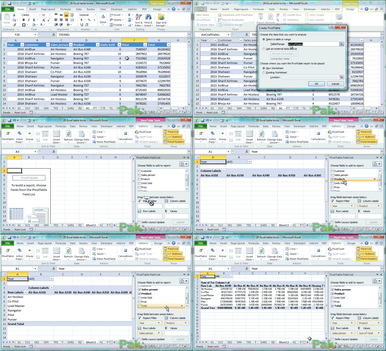
Now you have the pivot table done for you giving you the information how much revenue is generated by each sales person in each product.

But if you like to know how much sales are made by each sales person to each customer, you can find out that as well. This is what pivot tables are; swift easy results out of numbers. To get this information following these steps:

Step 1: Click anywhere inside pivot table so that pivot table field list appear again.

Step 2: From the column label box below, drag the products out of it by clicking and dragging it out. This will remove products.

Step 3: Drag customers from the list and drop it in the column label box.

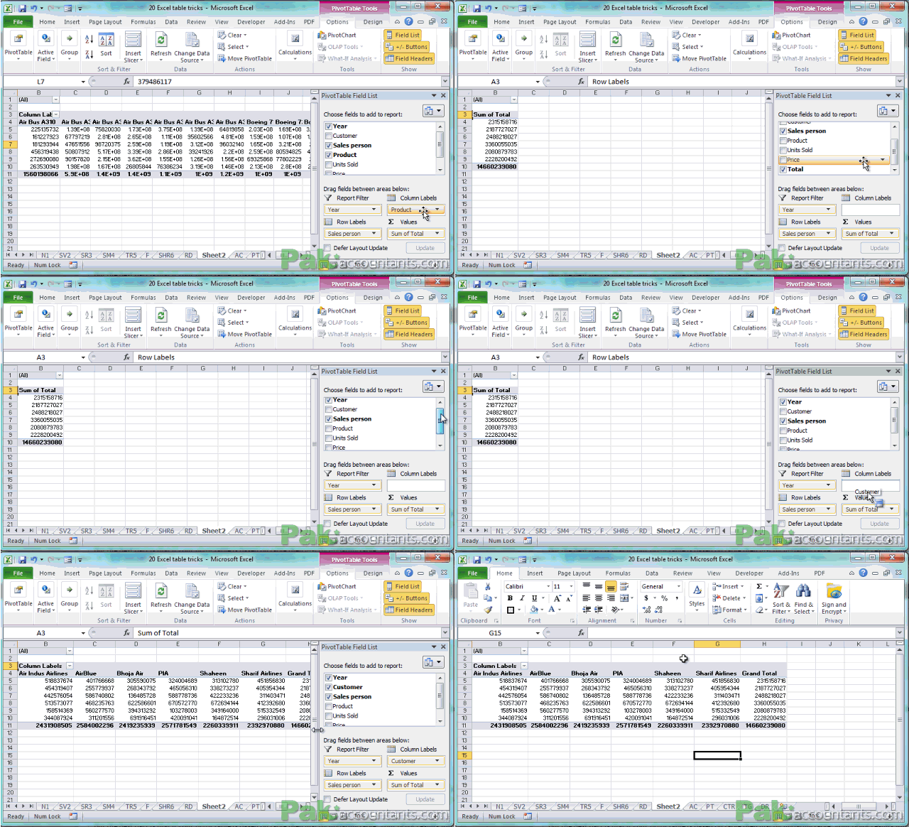
Your required report is ready giving you information about how much each sales person made from each customer.

But what if our sales data grows? Do we have to make pivot table again? Well if your pivot table was based on normal range then this might have been the case. But as our pivot table is based on table, therefore if you add new data to it and refresh the pivot table, the new data gets included automatically saving you the whole process of reconstructing the pivot table from scratch

Watch following animation where we included two new records with customers Lufthansa and Kamra, sales person: Hasaan selling Jango air crafts. Once refreshed pivot table includes newly entered data. FAN TABLE OUS!