Calculate Moving Average in Excel – How To

One of the ways to predict future is by observing where past is leaning. Trend analysis helps in forecasting the future based on past data. However, such data has the effects of different types of variations. With such variations its hard to conduct extrapolation and we need to get rid of them to get the core trend.

Financial analysts widely use moving average technique to determine hidden trends from set of data. And today we are learning how to do it using Excel starting with very basic and gradually discussing advanced uses.

One important aspect is interval used for average. It is simply the number of periods we are considering to average each time, lets say 3, and then move one period forward and take group of 3 periods again to calculate average. So if I have to show how its done have a peak at the picture. The first three numbers are done for you. The rest are done on the same basis. We want to achieve this with Excel and get to know some real life requirements.

Few things before we move forward:

1. Download this workbook so that you can also work along and apply the process discussed below.
2. In the beginning I am assuming interval of moving average is 3. We will get to have this variable later in this tutorial.

Case 1 – Using SUM function and ratio

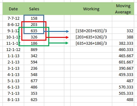
Very basic and requires manual work no intelligence on part of Excel. As I am assuming three periods to be averaged every time so we will start with the third figure in the data skipping first two and enter the following formula:

=SUM(C4:C6)/3

Drag the fill handle down to fill the whole range. Ignore the error mark.

Case 2 – Using AVERAGE function

Why even bother to first sum and then divide if we already have a builtin AVERAGE function. So starting from cell D6 as before using the following formula will give you the same result:

=AVERAGE(C4:C6)

Easy right? Lets take things up a notch!

Bonus: Auto Moving Average on data update

Before we move further lets configure our data in a way so that it can accommodate additional data by calculating moving average every time new transaction is entered. For this best possible way is to use Excel Tables.

Simply convert the range to tables by selecting and hitting CTRL+T. In my case I converted the data to tables first and then tried punching in the formula as discussed in Case 2 above. But funny thing happened, the formula was applied to the whole column on its own:

Now its up to us if we want to accept the way first two numbers are calculated. Sometimes we do accept it like this. But sometimes we want it to be empty and averages to start at the right interval. I will come this second requirement later in this tutorial. Its a simple workaround.

I forgot to change the name of table. Give it any name. I gave it MAv.

Bonus – Moving Average of latest quarter [Latest 3 months]

Now that our table can update and conduct calculations automatically if new data is entered. Another benefit is that it will save us lot of fuss and we do related calculates as well really easily. For example if we want to have a moving average of latest 3 period then following formula will help:

=AVERAGE(OFFSET(C4,COUNT(MAv[Sales])-3,0,3,1))

Lets talk about this a little. Above formula has three functions combined. AVERAGE, OFFSET and COUNT. Lets start with the innermost. Pro tip here! Always start with the innermost function as most of the time it will be calculated first.

COUNT(MAv[Sales]) – This part is counting how many rows our table has. I have given the sales column of MAv table to be checked. This will change as the data grows. But why that “-3”. I will come to that in a bit.

Few words about OFFSET, this function help us offset or skip specified number of rows and columns before fetching a cell or range of cells of certain height and width

OFFSET(C4,COUNT(MAv[Sales])-3,0,3,1) – Lets understand it by each argument:

Reference: C4 – this is the reference from where the excel will start measuring the offset

Row: COUNT(MAv[Sales])-3 – This part is calculating how many rows to skip from C4. In my example as of now there are 14 rows in total and 14-3 gives 11. So from C4 it will reach C15.

Column: 0 – Zero is mentioned here so no column will be skipped. So Excel will stay at cell C15.

Height: 3 – This tells how many rows should be fetched. 3 is mentioned so Excel will mark the rows 15, 16 and 17.

Width: 1 – This tells how many columns to be fetched. Here 1 is mentioned so its only column C. Therefore Excel will fetch C15, C16 and C17.

AVERAGE – Now that we have C15, C16 and C17 selected as a result of OFFSET and COUNT, AVERAGE function will calculate the average of these three.

Case 3 – Making average interval changeable

At the moment we have calculated the averages by selecting a particular range which is equal to number of periods we want to average. That has effectively fixed the number of intervals. What if we want to change it on the go? This is very much possible. Lets do this!

I mentioned the interval figure in cell G8 and named that cell “Int” by typing in the name box having the box active. Later used the following formula:

=AVERAGE(OFFSET([@Sales],-(Int-1),0,Int,1))

Now if you change the interval number, Excel will automatically calculate the moving averages based accordingly.

UPDATE: Neater OFFSET usage – Thanks to Brian

Though stories of comment sections should stay in comment section, but Brian’s version was a joy and I really liked the way it simplified the usage and still got the work done. So to applaud and thank I found no better way but to update the article with his suggestion added for life with his name!

Instead of proposed formula above that actually offsets the rows upwards from the given cell and then fetch the range downwards we can simply fetch the height upwards using negative argument. Following Brian’s suggestion the formula can be:

=AVERAGE(OFFSET([@Sales],,,-Int,1))

Case 4 – Adjusting average to accommodate Zero

Lets say our data may have zeros. And our client suggest that if it happens then immediately preceding value should be considered for average calculations skipping zero. For this our formula has to undergo some serious upgrade as follows:

=AVERAGE(IF(ISNA(MATCH(0,OFFSET([@Sales],-(Int-1),0,Int,1),0))=TRUE,OFFSET([@Sales],-(Int-1),0,Int,1),LARGE(OFFSET([@Sales],-(Int),0,Int+1,1),ROW($S$1:INDIRECT("S"&Int)))))

The above formula is an array formula and has to be entered by hitting CTRL+SHIFT+ENTER instead of simply ENTER stroke.

This is how worksheet is performing after I implemented the above formula:

Bonus – Hiding numbers for periods before interval completes

Better practice is to take only those moving averages when interval actually completes. For example if my interval is 3 then I cannot have a moving average before September 1, 2012 according to my data. So far it has not been causing any trouble but if data is stressed then it can through different types of errors, so its better to get rid of unrelated data.

So tweaking our formula a little more using another IF function can get us desired results:

=IF((ROW([@Sales])-3)<Int,"",AVERAGE(IF(ISNA(MATCH(0,OFFSET([@Sales],-(Int-1),0,Int,1),0))=TRUE,OFFSET([@Sales],-(Int-1),0,Int,1),LARGE(OFFSET([@Sales],-(Int),0,Int+1,1),ROW($S$1:INDIRECT("S"&Int))))))

Again, it is important to remember that above formula is an array formula and needs to be entered using CTRL+SHIFT+ENTER combination. And following is the result once updated:

Case 5 – Use builtin Data Analysis Toolpak

Yes! I kept the secret until now. I like to enjoy easy bits as reward at the end of hardwork!

To access data analysis tools you must have “Analysis Tookpak” enabled from Developer’s tab. Once enabled “Data Analysis” button will be available under Data tab in Excel ribbon.

This tool really simplifies the process as you just have to follow the instructions in the dialogue box and that’t it!

So here you have five cases to learn from. Definitely there can be hundred other real life requirements but I hope it will help you have a jump start and getting better at Excel!

Checkout the following tutorials as well to be better at Data Analysis:

1. Dynamic Common Size and DuPont Analysis Financial Statements in Excel
2. Excel chart of Top / Bottom “N” values using RANK() function and Form controls
3. Using Conditional Formatting to highlight range of percentages in Excel
4. Making Aging Analysis Reports Using Excel – How To
5. Excel for Accountants – 10 Must Read Tutotrials