Creating Scrollable data ranges in Excel – Excel Form Controls: Scroll Bars

If Excel ever had a tongue it surely would have told us that eating thousands of rows is as delicious for it as dunking oreos in milk for humans!

But we humans have another issue and that is we easily get tired of scrolling down especially if the list is so long as if it is emerging from the center of the earth. Things would be much more easy if we can scroll through the whole range but only a subset of data appears to make things easier to manage and interpret. What I mean is to have something like shown below:

Yes! It really is interesting and getting it is not so difficult either. So lets do it!

Step 1: First thing you need is to have your developer’s tab to be activated if its not already. Have a look at the following animation to understand the process of activation.

Step 2: Go to developer tab > controls group > insert button drop down > click scroll bar controls. This will change the cursor to plus sign enabling you to draw the scroll bar anywhere in the worksheet. You can choose to draw it horizontally or vertically. I will go with vertical orientation.

Step 3: Right click on the scroll bar > format controls. This will open up format control dialogue box.

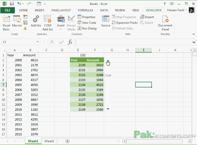
Minimum value: the minimum value scroll bar can generate. This is the starting point of scrolling. I had it set to 2.

Maximum value: the maximum value scroll bar can generate. This can serve as the last point of scroll. I had it set to 490.

Incremental change: lets you adjust how many cells scroll bar should jump if you click on arrow buttons. If it is 1 then it will jump 1 cell. If it is 10 it will jump 10 cells. I had it set to 10.

Page change: If you click somewhere in the scroll bar, it will act as page up or page down command. This value lets you adjust how many cells it should jump. I had it set to 100.

Step 4: In cell link mention the cell address where you want scroll bar to give output. This output will be in the form of numbers which we will help us use scroll bar. I linked cell E1 by mentioning $E$1 in the cell link input box.

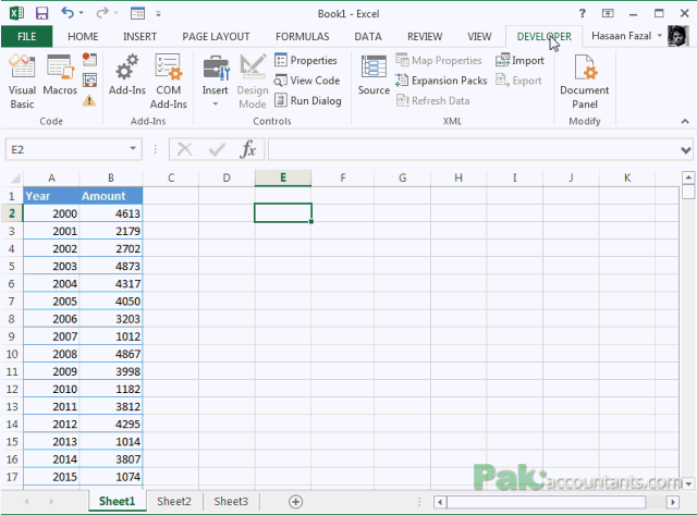
Step 5: In cell E2 give heading Years and in cell F2 Amount

Step 6: In cell E3 put the following formula and drag the fill handle down to cell E12:

=INDEX($A$1:$A$500,$E$1+ROW()-3)

The index function will be fetching only a specific value from the range A1:A500. The value to be fetched is dependent on the value in cell E1 which is linked to scroll bar and if scroll bar is moved the value in cell E1 will change too.

ROW()-3 argument is to automate the process even further and makes fetching value easier as we drag the formula down. We put this formula in cell E3 ROW() function helps us fetch the row value i.e. 3. But why ROW()-3? I leave that for you to solve. Let me know if you don’t get it in the comment box below and I will explain it 🙂

Step 7: Go to cell F3 and put the following formula and drag the fill handle down to cell F12:

=INDEX($B$1:$B$500,$E$1+ROW()-3)

Same thing as the formula in step 6 the difference is this formula is fetching the values from Amount column.

Step 8: Scroll it!

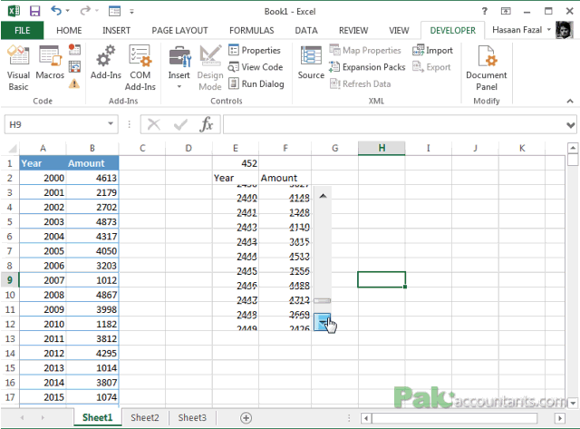
When you scroll, you will get the results of 10 years making it much easier for you to understand the data by having a subset out of the whole population.

Step 9: I figured out that the last value of the range which is year 2500 does not show up if I scroll down to very end. To fix it, I just need to adjust me max value in the scroll bar settings. I had the value 492 and to get one additional value listed I need to make it 493 and that will fix the problem.

So you have learnt another Excel form control and its basic use. Don’t forget to check out the following tutorials involving form controls:

1. Create Edgy To-Do or Check Lists with Check boxes in Excel + Shortfall calculator
2. Making Interactive Charts in Excel [How To]