First things first, this post is strictly for those who have Excel 2010 or later installed. But is this a warning not to read this post if you have older versions? NO! The intention is however, very opposite. I would really like that you must convince rather pressurize IT department of your company to have at least Excel 2010 installed. Believe me if you are still working on 2003, you really are living in days when the biggest invention was… a wheel!
Things have changed since 2007 and they changed even more with the release of 2010 version. Many things were dropped and many new were introduced. One of such new additions in Excel 2010 is Slicers or to be precise Pivot Table Slicers.
What are Slicers?
Long story short, these are same old filters but in 2010 they got plastic surgery and now they are so brave and bold that they got a new name, shape, options and even a new place inside pivot table contextual tab.
Technically slicers let you filter the data or slice the data by providing clickable buttons that can filter data once clicked. So it saves you some precious click effort as you don’t have to go fumble inside filter menu to do the same.
Can’t wait to have your hands on this and how to use it? Its just a click away 🙂
Pivoting with Slicers
Things you need – Prerequisites
Adding slicers to pivot table is really is pain free as you don’t have to dig deeper or do any kind of programming mumbo-jumbo. But you do need a pivot table or a data of which you want to make a pivot table. So basically it adds to convenience while working with pivot tables and it is not a stand alone feature.
Adding slicers
Open the excel workbook you downloaded and make sure Pivot Table worksheet is active.
Step 1: Have an active cell inside pivot table. If you don’t have one then create a pivot table to awake slicers. To learn how to create a pivot table you can read Part 2 of two part series on pivot table which has been loved by many since day 1.
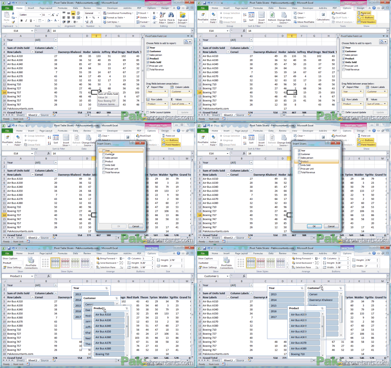
Step 2: Once you have a pivot table and you have an active cell inside it, go to the contextual tab named Pivot Table tools and click Options tab under it. In Sort and Filter group you have slicers button. Click it!
Step 3: A new window appears containing some options which you can select by checking them. These options are actually the columns of your data and are the same elements you used to create pivot report. Make the selections for which you want slicers to activate. If you are undecided then check; years, product and customer and click OK.
Step 4: You will get three new soft windows hovering above pivot table.
Step 5: You can click and hold titles to move the slicer windows around and arrange them as per your work space.
Following animation shows how to carry out above steps:

Using Slicers
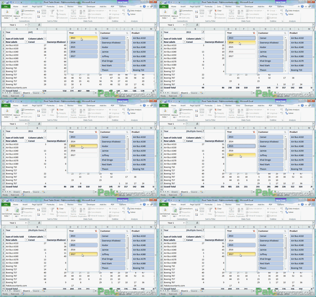
Play with the buttons and you will get the data filtered for you in one click.
For example:
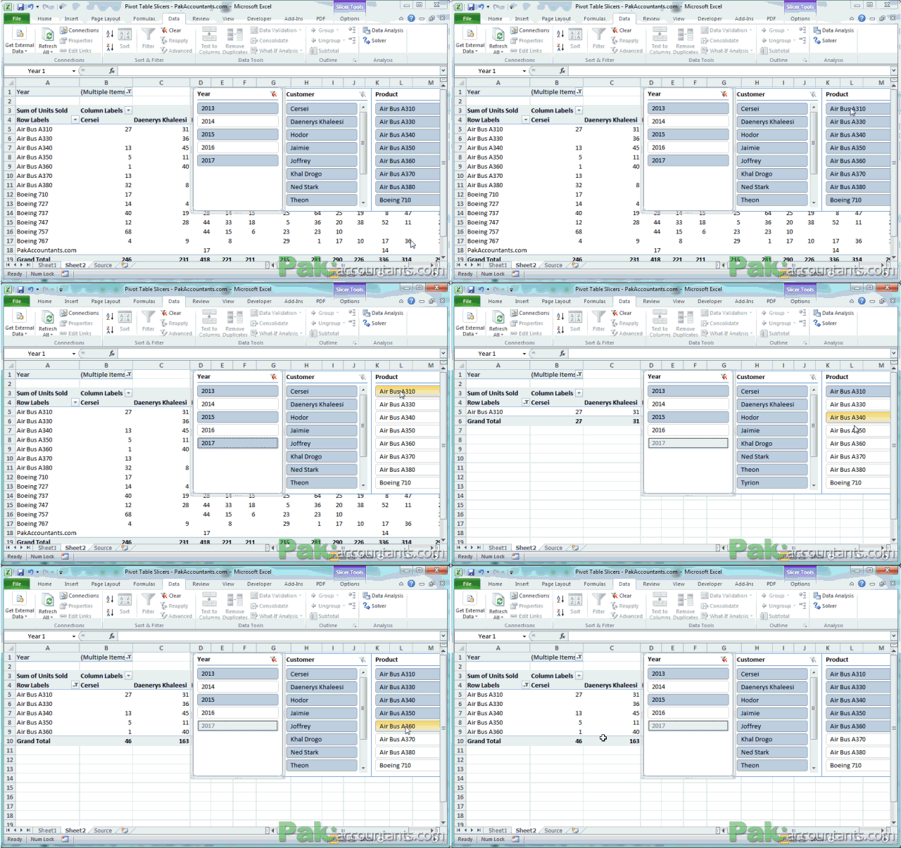
To filter data only for year 2013 click 2013 button in Year window and pivot report will display results from year 2013 only. You can sub-filter data further using slicers in other two windows. For example, click Air Bus A310 in product window and pivot table will filter and report only the results relating to product Air Bus A310 by all customers for year 2013. To filter it further and to show results only for one customer, lets say Theon, click on its name in Customers’ slicer window and report will filter further.

How quick was that! With just three clicks you have filtered the data for one customer, one product for one year. Without slicers you would have to filter it one by one for each field going in filter options menu. This is for sure a great productivity enhancer.
To clear filters simply click the funnel icon with red cross on it at the top right corner of every slicer window. This will clear the filter from one category only. To remove filters from other categories you will have to click the remove filter icon separately.
Having the slicer window active, you can use Alt+C shortcut to remove filter from that particular data group or category. To clear filters from all at once then click anywhere on pivot table and hit Alt+A+C. Alternatively you can go to Data Tab > Sort and Filter group > Click Clear button

So what you say? You don’t have to be a ninja to slice so easily in Excel after all 🙂
Bonus Tip – Selecting multiple slicers
In normal filter application, you have option to select multiple items out of category. In slicers you have buttons but you can still select multiple slices by using Ctrl or Shift key combos. Following examples help you carry that out easily.
Multiple slicers selection with CTRL key
Suppose you want to select year 2013, 2015 and 2017. You can do this by pressing and holding down Ctrl key on the keyboard and use mouse to click 2013, 2015 and 2017 buttons. But make the first click on 2013 without Ctrl key pressed then press and hold the Ctrl key down to make multiple selection. Notice that 2013, 2015 and 2017 are colored whereas rest are colorless.

If you press and hold Ctrl key even before first click then Ctrl key will help you exclude the years from result. Notice in the following animation the years you clicked got deselected. Its the opposite of what we did before.

Multiple slicers selection with SHIFT key
The working of Shift key in this situation is as normal i.e. if you press and hold Shift key and click two areas the area or items in between also get selected. Similarly in our pivot table if you want to select all products from A310 to A360 (both included) then click A310 once and then press and hold down Shift key on the keyboard and then click A360.

I hope many of you must be thrilled to learn this amazing new feature in Excel 2010 or waiting to have their hands on if they are currently not working on 2010 version. Do let me know how you are using slicers in your daily work. These can be put to some really advanced levels which I have planned to discuss in later posts on Pivot Tables.
Don’t forget to checkout our other articles on Excel Pivot Tables here

Another one of your great posts, keep up the good reads…