Comparing two columns to highlight Duplicates in the same row – Excel Conditional Formatting

Back to Excel after a long time. But now starting to relax a little as course is concluded for many subjects I teach. I really missed my Excel community and I really want to thank each and everyone of them that they have not given up on me. Love you all!

During my break from Excel I got loads of questions on different aspects of Excel and I really mean loooooooadddsss of them through facebook Excel page, emails, twitter, sms and you name it. And some of them really got my attention but I am going to start with the latest of all which also happens to be the easiest of all.

Scenario debrief – Understanding problem

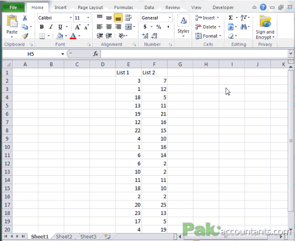
Basically we have two lists in two columns with numbers and some numbers are repetitive either in the same list or in the other list. But we want to highlight only those that are not only in the other list but also in the same row. For example if cell A1 of column A has 5 and if cell B1 of column B also have 5 then its a duplicate.

Having 5 in A1 and B2 will not be considered a duplicate as the rows are different.

Approach debrief – How to solve it

Our basic aim is to compare the list in a way that we can identify the duplicates. The best is to highlight them using different colours so that duplicates stand out from the rest (i.e. the ones that are not duplicate).

To do this we will use Excel’s in-house feature called Conditional Formatting. Now as the name is suggesting, this let you format the cells or range of cells if certain condition (or conditions) is fulfilled. So lets see how is this done in few down to earth easy steps.

Using conditional formatting to highlight duplicates

Step 1: Open the tutorial file. You can download it from the link above mentioned in the red box.

Step 2: Select column E either using mouse by hovering mouse cursor over cell E1 > click left mouse button and hold it > drag mouse until the selection covers the content in cell E25. You can also do this via keyboard by selecting cell E1 > Press and hold Ctrl+Shift and pressing Alt Down arrow key. This will instantly select the whole range.

Step 3: Go to Home tab > Styles group > click Conditional formatting drop down button > and from the list select new rule

Step 4: A new formatting rule box will box pop up. From this select the second bullet “format only cells that contain”.

Step 5: From below click the second drop down list to select “equal to” and in the range box to its right type

=F2

Step 6: Underneath you have formatting options. By default no formatting is done, therefore to separate the duplicates it would be good to have different cell fill colour. To do this click “format” button and a box will colour options will be displayed. Select any colour that you like or the one that goes with your worksheet theme. Click OK and then OK button again. This will highlight the numbers that are duplicate in column E.

Following animation help you understand how above steps are carried out:

Step 7: Repeat the same process from step 3 to step 6 for column F values but this time when you are mentioning the cell address in the range box for “equal to” you will mention cell E2 as now you want to compare the values of cell F2 with it. It will be good if you with same formatting as you did before as it will create smooth duplicate highlighting.

Bonus tip: Sorting/Filtering/Separating the duplicates using colours

Once you have identified the duplicates using the technique above you can filter out the duplicates pretty easily using colours. Lets see how this is done:

Sorting using colours

Step 1: Select both the columns by having an active cell within any of the columns and hitting Ctrl+A.

Step 2: Hit Ctrl+Shift+L to enable Data filter and you can know if this is enabled as the cells E1 and F1 are going to have small arrows arrows pointing downwards in a box.

Step 3: Click the filter arrow of any coloumn and from the menu select filter by colour and from sub-menu select the colour. This way the coloured cells will appear first in the list i.e. ascending order.

Filtering using colours

Filtering is almost the same as sorting using colours. But this time after you click arrows go to “filter by colours” option and select the colour. And only those cells that have specific colour will be displayed.

Separating using colours

If you want to copy the duplicate values then after filtering done, you need to do one additional step. However, its not really as simple as selecting copying and pasting as if you try to select the filtered result using the normal way it will select even the results that are filtered out.

To select only filtered results you have to select only visible cells. To do this after you have applied the filter. Hit Alt+; shortcut combo and it will select only the visible cells. Now you can copy and paste just the filtered results (which are duplicates).