ABC analysis is an inventory management technique in which stock is classified in usually three categories on the basis of their importance. Such classification help management to concentrate their efforts on such products that are more important in terms of revenue they are generating, cost or any other measure entity is using to judge importance.
You can read in detail about ABC analysis here: What is ABC Analysis?
In simple words, ABC analysis categorizes inventory in three categories:
- A – most important
- B – important
- C – less important or marginally important
Lets say we are measuring importance in terms of revenue generated by the product. It is usually observed that 10-15% of the products offered by the entity generate 70-80% of the total sales revenue. With Excel classifying inventory in this fashion is really simple. Lets say:
- Products that generate 70% of sales be categorized as A
- Products that generate next 25% sales be categorized as B
- And products that generate rest of the revenue which is 5% are categorized as C
In short:
0% – 70% – A
70% – 95% – B
95% – 100% – C
This is what we are after in this tutorial after we done understanding how Excel helps us in categorizing products based on given data:

ABC Analysis using Excel
Step 1: Open up Excel and have above information of classification in cell A1:
| 0 | 0.7 |
| 0.7 | 0.95 |
| 0.95 | 1 |
Step 2: Copy the following data and paste it in your worksheet in cell A5
| Product | Amount |
| Sesme – 1 | 20,000 |
| Sesme – 2 | 17000 |
| Sesme – 3 | 14450 |
| Sesme – 4 | 12283 |
| Sesme – 5 | 10441 |
| Sesme – 6 | 8875 |
| Sesme – 7 | 7544 |
| Sesme – 8 | 6412 |
| Sesme – 9 | 5450 |
| Sesme – 10 | 4633 |
| Sesme – 11 | 3938 |
| Sesme – 12 | 3347 |
| Sesme – 13 | 2845 |
| Sesme – 14 | 2418 |
| Sesme – 15 | 2055 |
| Sesme – 16 | 1747 |
| Sesme – 17 | 1485 |
| Sesme – 18 | 1262 |
| Sesme – 19 | 1073 |
| Sesme – 20 | 912 |
| Sesme – 21 | 775 |
| Sesme – 22 | 659 |
| Sesme – 23 | 560 |
| Sesme – 24 | 476 |
| Sesme – 25 | 405 |
| Sesme – 26 | 344 |
| Sesme – 27 | 292 |
| Sesme – 28 | 248 |
| Sesme – 29 | 211 |
| Sesme – 30 | 179 |
| Sesme – 31 | 152 |
| Sesme – 32 | 129 |
| Sesme – 33 | 110 |
| Sesme – 34 | 94 |
| Sesme – 35 | 80 |
| Sesme – 36 | 68 |
| Sesme – 37 | 58 |
| Sesme – 38 | 49 |
| Sesme – 39 | 42 |
| Sesme – 40 | 36 |
| Sesme – 41 | 31 |
| Sesme – 42 | 26 |
| Sesme – 43 | 22 |
| Sesme – 44 | 19 |
| Sesme – 45 | 16 |
| Sesme – 46 | 14 |
| Sesme – 47 | 12 |
| Sesme – 48 | 10 |
| Sesme – 49 | 9 |
| Sesme – 50 | 8 |
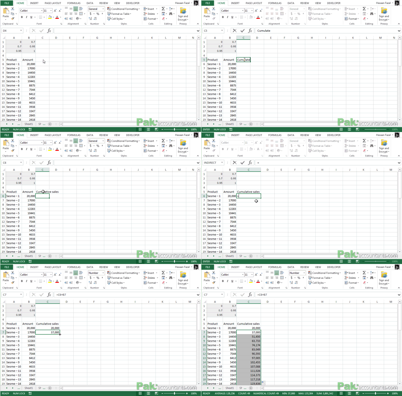
Following animation will walk you through the process:

Step 3: Go to cell C5 and make a heading Cumulative revenue and in cell:
- C6 put the formula: = B6
- C7 put the formula: =C6+B7 and drag the fill handle down to cell C55 or simply double click to populate the cells down.

Step 4: Select all cells from A6 down to A55 using mouse or keyboard.
Tip: You can do this quickly by having an active cell A6 and Press and Hold Shift + Ctrl keys and press Down arrow key. And hitting Ctrl+Backspace to come back up to active cell.
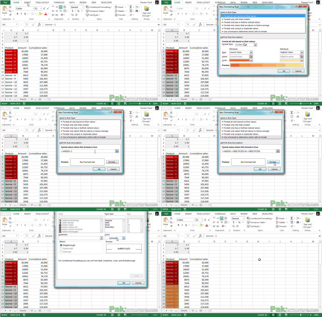
Step 5: Go to Home tab > Styles group > Click conditional formatting drop down button > click new rule > From the dialogue box click use a formula to determine which cells to format > Put the following formula:
=IF(C6<=$B$1*$C$55,TRUE)
Make any necessary changes. I went with Red fill and white font color for the first category i.e. A.

Now we will repeat step 5 two more time to add two more conditions for category B and C. Just follow along:
Step 6: Go to Home tab > Styles group > Click conditional formatting drop down button > click new rule > From the dialogue box click use a formula to determine which cells to format > Put the following formula for category B goods:
=AND(C6>=$B$1*$C$55,C6<=$B$2*$C$55)
I chose dark orange color with white font to make category B stand out.
Following animation will help walk you through the steps:

Step 7: Go to Home tab > Styles group > Click conditional formatting drop down button > click new rule > From the dialogue box click use a formula to determine which cells to format > Put the following formula for category C goods:
=AND(C6>=$B$2*$C$55,C6<=$B$3*$C$55)
I chose parrot green color with white font to categorize C type products.
Following illustration will prove helpful:

Step 8: Sometimes you have to really tell Excel in what order to apply the conditional formatting as it really messes up. But sometimes it tends to understand. But I wasn’t so lucky this time.
So just to be on the safe side we better have our category A formatting at the top, Category B formatting condition in mid and Category C condition in the last as the following illustration shows:

Now you have three bands of colors.
- Product 1 – 7 are category A products
- Product 8 – 18 are category B products
- Product 19 – 50 are category C products
Coming back to our ABC concept. As we have total 50 items on sale and just by looking at the colors we can observe that just 7 are generating 70% of total sales of the entity. If we take a ratio of 7 over total products of 50 it comes up 14%. In other words only 14% of all the products on offer are making 70% of total revenue of the entity.
On the other hand we have 30-31 products in category C and this makes up 30/50 x 100 = 60% of total products and generating just 5% of total revenue.
Understanding this fact, entity should reinforce their efforts towards those 7 products that are in category A and be very vigilant towards their fluctuations as it will hurt revenues significantly. On the other hand, although Category C items are more in terms of count but still not nearly as important as category A products.
So as you understand how this analysis helps management make better decisions and Excel let them take these decisions in no time by making it super easy to get the right information available.

Thank you for the rich article, esspecially for GIF animations which are really helpful and fast.
Love this!