One minute Excel Tutorial – Split Margins / Split Window / Split Screen / Split View

Hasaan Fazal

Data is meant to be long and stretched but data segment that we want to attend is sometime too scattered that we cannot help scrolling. But this can be catered if we can somehow split the work space in two independent regions and then observing the two spaces. In excel this is easy with split window feature. It is also referred as split sheet, split screen or split margins etc.

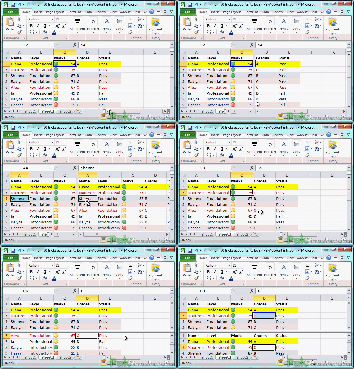
What it basically does it divides the worksheet in 2 or 4 quadrants and you can scroll each quadrant independently of the other to review data on same worksheet. This feature comes with many names like: split margins, split window, split screen, split view, split, split spaces, split workspace or split anything you like to call it!

Table of Contents

Divide and rule!

You can achieve this either

using mouse; or
command button from ribbon.

Split window using mouse

Just above the vertical scroll bar under formula bar you can see a small rectangle. Move your cursor above it press left click and hold and move mouse to the center of the worksheet. Voila! there you have it. Your one worksheet split up in two independent horizontal work spaces. Similarly, at the right of bottom scroll bar same rectangle exists. Repeat the process and it will split the work spaces vertically. Combining two splitters you can achieve 4 independent quadrants or work spaces.

You can adjust the split bar where you want it by hovering mouse above split bar then press and hold left click and drag. The split bar every time jumps one cell i.e. either one row or column.

You can disable the split view by dragging the horizontal split bar to top or bottom of screen. For vertical bar drag the split bar either to the very right or left of the screen. To quickly close the divider, double click the split bar itself and worksheet will revert to normal view.

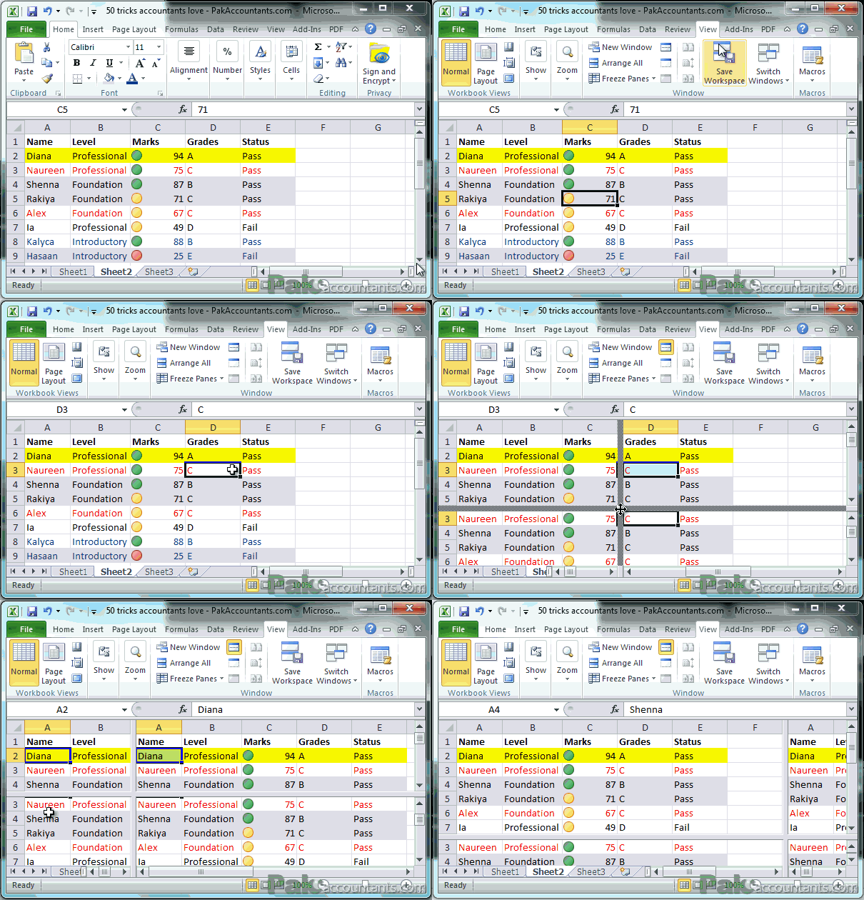
Split window using command button

You can have it done using ribbon above. Click View tab and in Windows group click Split and the split margins will appear at the top left corner of the active cell.