Before in Excel tips we learnt about Custom Lists feature in Excel and how to use it to sort and have custom autofill series. In our example we sorted the sales data using our own criteria of cities that was not alphabetical. That helped us having data of cities first that are more important to us then sales data from other cities. However, what if we want to have data sorted like this:
- First sort the data on the basis of cities using our custom lists
- Second sort the sales data sorted in descending order i.e. showing highest sale first for each city
This is achieved using Excel’s multi-level sort feature also known as multi-column sort. It comes as additional option with sort feature of excel which you can access through sort dialogue box. We will explain how to do it step-by-step in this debrief.
Note: To keep things simple we are adding just one additional criteria, however, you can have as many as you can to help you get the desired output.
Sortin Time!
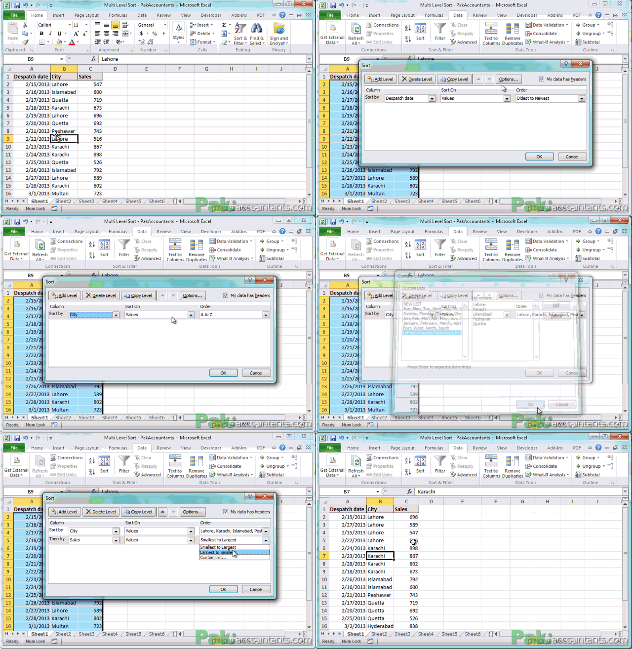
Step 1: Consider the data that you want to sort. Either make the selection out of range of data or have an active cell within specific range of cells.
Step 2: In the ribbon above click Data tab > Sort and Filter group > Sort button
Step 3: In the sort dialogue box that appears, from the sort by drop down select City and from the order drop down select custom list. Don’t change sort on drop down selection and keep values selected. To learn how to make custom lists read: Custom Autofill series and Custom sorting with Custom lists in Excel
Step 4: Custom list dialogue box will pop up. From this make the selection of custom list we have already created. Click OK
Step 5: Click Add level button at the top in the sort dialogue box. This will add another level of sort or simply criteria.
Step 6: In the level just created, from then by drop down select sales and from order drop down select largest to smallest. Keep “values” selected in the sort on drop down. Click OK
Following animation walks you through all the six steps discussed above:

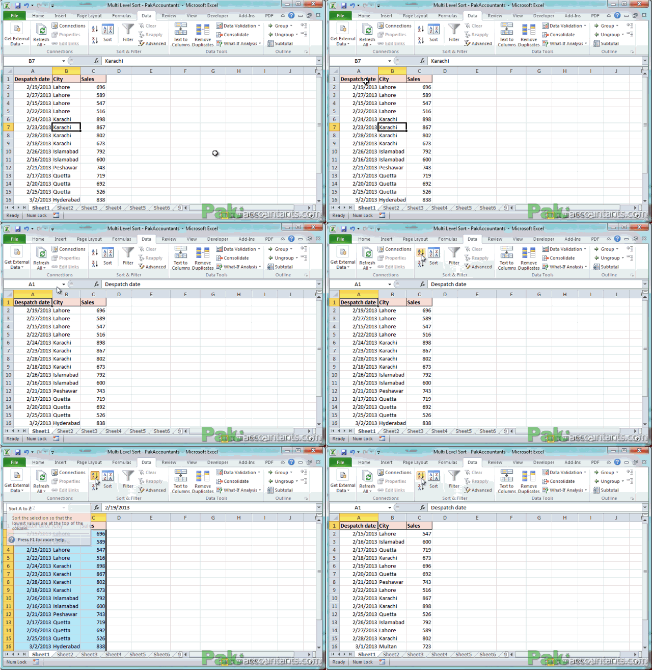
And here you have data sorted by cities in the order you specific in your custom list and then the sales reported in descending order for each city.
How multi level sort works:
Each level acts as sort run in excel that are executed in the order we specify i.e. the order in which excel to sort. As we have two levels city criteria first and sales criteria second. Therefore, excel will first sort excel’s data on the basis of city. Once done excel will sub-sort the data in the sales column for each city by showing highest sale first.
Bonus Tips:
- If you want to change the order of criteria application then you can do that simply by selecting each level and clicking arrow up or arrow down to move it above or below other levels. You can also use shortcut keys Ctrl+Arrow Up to move up and Ctrl+Arrow Down to move level down.

- You can sort the data on columnar basis or row basis. To learn how to do this read: How to sort Rows horizontally left to right instead of Columns vertically top to bottom in Excel
- Care must be taken for data that does not have headers. If it has headers then check the option “My data has headers” in the top right corner of sort dialogue box. If it does not than uncheck otherwise first row will be excluded from sort function.
- If you are sorting on row basis then “my data has headers” option is not available and you manually have to exclude the first row if it has row headers while selecting data before sort.
Caution:
Sorting is a permanent movement in data. Unlike filter which temporarily moves the data according to criteria and puts data back once criteria is cleared. Only possible way to rearrange data back is by Undo or having a column dedicated for this. For example before sort you can have serial number column and can revert to original order of data by arranging serial number column. Like in our example, earlier the data was arranged in chronological order. If we want to revert to original order we just sort the dates in ascending order.

Liked it? Pin it!

