Prepare (Normalize) the data for Pivot Tables using Power Query

Pivot tables is a love of life for many Excel heads for its ability to move elements of reports easily is pure awesomeness. Pivot table has greatly improved since improv. But it still has limitations. And one of such is source data needs to be in specific structure to get the most of pivot table muscle.

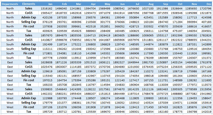
Data structure as given below is a common sight:

There is nothing wrong in the data itself. Its good and is kind of mini-report in itself as you can easily see the values of different elements for each month across rows and different values of each element across the column. It can suffice many data requirements.

We can even make pivot tables with this data, Excel won’t go bananas if we execute a pivot table command over it, however we won’t be able to use different capabilities of pivot tables effectively as our data is scatter along columns AND rows its a cross type data which pivot table don’t like.

The two important requirements for source data meant for pivot table are:

1. data must be arranged in columns i.e. from top to bottom. No property should be put in row to form intersections of data sets.
2. Similar data or data of same type should be put in one column with its name as column header.

If you see the data above again, we have months from left to right and we have departments and elements of financial information in one column. In short it has all the problems we never wanted.

For pivot table to work best the above data has to arranged in columnar format as given below:

Calling Power Query to the rescue

Believe it or not using power query is just like drawing pokemon power card or that hidden beyblade that you had in your pocket all the time and you still facing rants with calm face! Or if you are from ancient times then invoking power query is just like Liono’s assemble cry and all the brains and muscles come together to face the dreaded enemy – the Data!

First and foremost you need to install the power query add-in into your system (before you can go all thunder! thunder! you need the sword right?). To download visit this link. Once downloaded, use the installer to get the add-in working. It will show up as a separate tab in Excel. Let me know if you face problem in this regard.

By the way it requires Excel 2010 or 2013 for some reason. But for what reason on earth are you still using older versions? Come on! 2013 is too cool to be ignored!

I know some organizations are too lazy to understand it so I will explain alternative methods to correct the data structure in future posts if power query is not available to you.

Coming back to our case, once installed and ready follow these steps to correct the data we are considering:

Step 1: Select the range and convert it to table by pressing Ctrl+T.

Though it is not needed to execute power query command as it will automatically do it for you as the first step.

Step 2: Have an active cell inside the table, click Power query tab > Excel data group > click from table button. It will load the table in query editor window.

Step 3: Select the columns from Jan through Dec by holding down Shift key on the keyboard and using mouse to complete the selection.

Step 4: Go to Transform tab > any column group > click unpivot columns.

BANG! Your data is restructured with all the months name in columns in the blink of an eye. Double click the the attribute heading and name it Month.

Step 5: Now select Element column and Value column together holding down Ctrl key this time.

Step 6: Go to transform tab > any column group > click pivot column button this time. A message will popup click OK.

Here you can see the preview of your data ready to be saved.

Step 7: Click Home tab > click close & load button. A new worksheet will be inserted with the table structured and all ready for pivot table work.

If you liked this tutorial you will love other Pivot tables tips & tutorials too:

1. Excel Pivot Table tutorial for Absolute Beginners: Creating your First Pivot Report [2 of 2]
2. Running Totals and Running Balance with Excel Pivot Tables – How To
3. Excel Pivot Tables – Grouping Dates by Week Within Months, Quarters or Years – Workaround
4. Making Sales Dashboard using Excel Slicers – How To