For reporting purposes sometimes its elegant to show dates as quarters of the year instead of months. It helps managing clutter in a large set of data. As much as I wish there was a way to do it using custom number formatting Excel doesn’t have such ability as such and thus we have to look somewhere else.
But we can surely do it using Excel formulas. And here is what we are learning today:

Formatting Dates as Quarters – Thoughts!
I personally like the use of TEXT function to format year part of the format as it gives me much more flexibility then using using simple YEAR function.
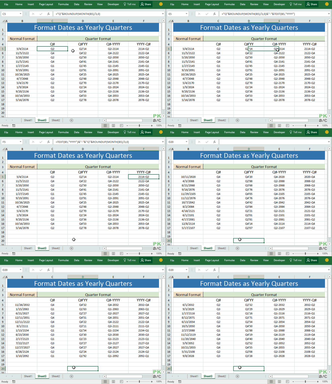
Here is one example where I have list of dates with a normal format and I want to format them in four different ways with formulas I used to get the required format with the date value in cell B5:
Q# e.g. Q1:
=”Q”&ROUNDUP(MONTH(B5)/3,0)
Q#’YY e.g. Q2’17
=”Q”&ROUNDUP(MONTH(B5)/3,0)&”‘”&TEXT(B5,”YY”)
Q#-YYYY e.g. Q3-2018
=”Q”&ROUNDUP(MONTH(B5)/3,0)&”-“&TEXT(B5,”YYYY”)
YYYY-Q# e.g. 2007-Q4
=TEXT(B5,”YYYY”)&”-“&”Q”&ROUNDUP(MONTH(B5)/3,0)
Here is the final result and you can see that format stays intact even if the dates change:

How is it working!
Lets take one of the formulas and understand how its working and all three examples will make sense. So here it is:
=”Q”&ROUNDUP(MONTH(B5)/3,0)&”-“&TEXT(B5,”YYYY”)
There are four functions at play here:
“&” connector: short-hand application of CONCATENATE function and is helping make a text string by connecting the output from several functions and manual input of “Q” at the start.
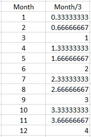
MONTH: helping us find the month figure in the date mentioned in cell B5 and then dividing it by 3 to determine the quarter. Surely it can result in decimal figures as following:

ROUNDUP: to cater the challenge of decimal figures I wrapped the result of MONTHS()/3 in ROUNDUP function and ask it to round up to zero decimal place thus a value with decimal portion greater than 0 will be forced to become whole 1 giving us the right quarter number:

TEXT: this function help us not only fetch the year portion of the date but also format the way we want. You can see in second type I used “YY” that rendered us only last two digits of the respective year number. And if “YYYY” is used it helped us get the full year number.
And again all this is connected together using “&” connector to give us one text string.
Here is the pictorial explanation of steps:


Can you help me on formula for fiscal year format.
=TEXT(B5,”YYYY”)&”-“&”Q”&ROUNDUP(MONTH(B5)/3,0)
Hello the below formulaes are not working and giving an error #NAME ? . could you help me on this
Q# e.g. Q1:
=”Q”&ROUNDUP(MONTH(B5)/3,0)
Q#’YY e.g. Q2’17
=”Q”&ROUNDUP(MONTH(B5)/3,0)&”‘”&TEXT(B5,”YY”)
Some more methods: how to calculate the quarter to which a month belongs
Suppose the date is in: C2
Method # 1:
=INT((MONTH(C2)-1)/3)+1
Method # 2:
=ROUND(ROUNDUP(MONTH(C2)/3,0),0)
Method # 3:
=MROUND(CEILING(MONTH(C2)/3,0.5),1)
Method # 4:
=ROUND(CEILING(MONTH(C2)/3,0.5),0)
Method # 5:
=ROUNDUP(ROUNDDOWN(MONTH($C2)/3,2),0)
What would be a formula if April, May, June were the first quarters??
For that you can either do with or without helper column. First you will have to adjust the month numbers to go according to custom fiscal year and then divide the month numbers by 3 to get the correct quarter numbers.
For helper column with adjust months in your case with date in cell A1:
=IF(MONTH(A1)>3, MONTH(A1)-3, MONTH(A1)+9)
In another helper column simply divide the adjusted month number with following formula with adjusted month in cell B1:
=ROUNDUP((B1/3),0)