Making Aging Analysis Reports using Excel Pivot Tables – How To

Last time when I discussed preparing aging analysis in Excel, I used formula approach to do it. I used the combination of IF and TODAY functions and then used conditional formatting and sparklines to add visual aids to the analysis. Here is the preview of it:

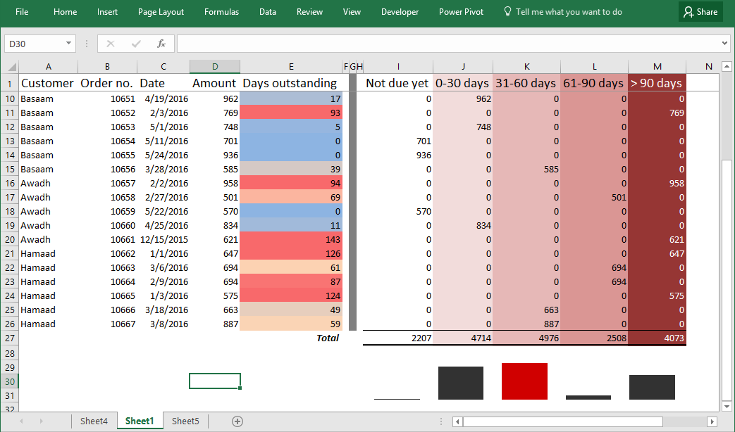
This time however, we will learn how to achieve the same report but with pivot tables. Pivot tables will not only save us from writing different formulas but also make it dynamic and we can extract different types of reports and not stuck with just one format. In short, pivot tables make almost everything crazy fast! And after today’s tutorial this is what we will get:

Nice, clean and above all, dynamic!

Before we move on, if you are new to aging analysis and want to know the basics then have a read of this concise article:  What is age, aged, ageing or aging analysis?

Watch the Aging Analysis free tutorial – Step by step

Understanding the data and requirement

So what we have is a list of customers each with multiple orders under their name with different invoice dates. What we want is to make a schedule so that we invoices are arranged coloumns as follows:

• Not due: The invoices which that has not fallen due yet
• 1-30 days: The invoices that are past due for days between 1 to 30 days.
• 31-60 days: The invoices that are past due for days between 31 to 60 days
• 61-90 days: The invoices that are past due for days between 61 to 90 days
• >90 days: the invoices that are past due for more than 90 days.

Understanding the approach

Unlike last approach I will be skipping “Days outstanding” column as its not needed if we have the analysis of invoices as “Not Due”, “1-30” and so on. Also as we are employing pivot table technique, there a new step involving VLOOKUP for approximate match will be part of the discussion. So lets get started.

Step by step: Debtors’ Aging report in Excel using Pivot tables

Step 1: Add a new column, give it a heading “Status”. In our case it will be column F. In this column we need to put if payment is “Not due” or “1-30 days” etc.

Step 2: Anywhere in the worksheet, lets say in column J and K give heading “Range” and “Status message”. And put the content as shown in the following figure:

Basically for invoices not fallen due yet, we will have 0 days and for that we want to fetch a status message of “Not due”. Similarly if invoice is due for, suppose, 14 days then message “1-30 days” will be printed in relevant cell. And we will do both tasks i.e. calculating days due and status message using single formula.

Step 3: Select the data in range and status message and go to name box and punch “strange” or any other unique name. This will this data range a name that we can use in formula.

Step 4: Select the debtors’ data and hit Ctrl+A this will select the whole range of data, hit Ctrl+T to change the range to excel table. This will help in making the base data dynamic. So that if we add more transactions to our data, pivot table will automatically take care of it and updating the report on the go!

Step 5: Put this formula in ‘Status’ column to determine the relevant message:

=VLOOKUP(IF(TODAY()>[@Date],TODAY()-[@Date],0),strange,2,TRUE)

Above formula is a combination of IF and VLOOKUP. Starting with the inner most function lets take a minute to understand what is it doing:

IF statement is checking if today’s date is greater than the date mentioned in relevant cell of ‘Date’ column of the table (which will be true if invoice is already due), then calculate the difference, otherwise return “0” meaning its not yet due.

Once the result of IF function is obtained, it is fed as “Lookup value” to VLOOKUP function and this function then determines the status message by going to range named “strange”. Now here lies another trick. First invoice, for example is due for 17 days now, VLOOKUP will go to the first column of “strange” range. Now it has either “1” or “31” in the column. As VLOOKUP is set to fetch “approximate” match (check our formula has TRUE argument), therefore, it will settle with the smallest amount of the match i.e. “1” and fetch the value from corresponding cell of column 2 and thus a message “1-30 days”.

Step 6: Select the table by having an active cell within the table and using Ctrl+A shortcut. Go to Insert tab > tables group > click pivot table button > Click OK. This will insert a new worksheet with pivot table.

Step 7: Drag the “Order no.” field to rows box, “Status” field to column box and “Amount” field to values box. TADA! You have the report ready! OK! Not quite yet, we need to do some shifting and make few formatting changes.

Step 8: There are few columns that needs to be shifted, you can easily do so by selecting the heading and dragging the edge of highlighter (using left mouse button, press and hold while dragging) and dropping it at the right point.

Step 9: Having an active cell within pivot table, go to design tab > layout group > click grand total drop-down button > click “On for columns only”.

Step 10: Go to Design tab > layout group > click layout drop down button > click show in out line form.

Following animation shows all the steps mentioned above:

This is exact same report that we got but using formula here. But this time we have some more flexibility. Suppose we want to know how much each customer owes us and in what time bracket. Think done boss!

Just go to pivot table, drag the order number field out, and drag the customer field in the row box. Go to design tab > layout group > grand totals > on for rows and columns.

And BINGO! Any body did the stopwatch here? No? No one?

Now you know how much each customer owes you and in what time bracket they owe you how much in today’s date.

After a bit of formatting touches this is how it looks:

Not forgetting the dynamic part, suppose there is a new customer named “Cheeky customer” to whom transaction of 7622 was made that is due by August 6, 2016. Now if you put this data in the source table and refresh the pivot table, the aging analysis report will update automatically as shown below:

So here you have it; a fast, dynamic aging analysis report using Excel pivot tables!

Don’t forget to check out following tutorials as well:

1. Dynamic Common Size and DuPont Analysis Financial Statements in Excel
2. Making Cash flow summary in Excel using Pivot tables with data on multiple worksheets
3. Budget Vs Actual – Analyzing Profit and Loss Statements in Excel using Pivot tables
4. Making Profit and Loss Statements in Excel using Pivot tables