In any financial model (forecasts or variance analysis) the idea is to derive expectations where business will end up if particular set of assumptions (scenario) prevails. These are basically calculations that help the decision making process.
Excel provides the necessary flexibility in designing such models. As calculations are based on assumptions, it is much easier for us to understand the effect of change in assumption and how the business and its resources will react.
Today we are looking at a simple example to understand how Excel can help us make Capital Expenditure forecasts and calculating net book value (NBV) each year using Excel formulas.
Scenario
We are required to make calculations with following information provided:
The forecast capital expenditures are as follows:
| Years | Capex |
| 2015 | 81 |
| 2016 | 55 |
| 2017 | 95 |
| 2018 | 13 |
| 2019 | 67 |
| 2020 | 18 |
| 2021 | 54 |
| 2022 | 58 |
| 2023 | 22 |
| 2024 | 86 |
| 2025 | 58 |
| 2026 | 97 |
| 2027 | 83 |
| 2028 | 21 |
| 2029 | 59 |
| 2030 | 71 |
Inflation rate of 5% per annum is expected. The useful life of asset is 5 years and thus fixed assets are depreciated on straight line basis over 5 years.
Clearing the approach
We need to do the following:
- Adjust the capital expenditure amounts for inflation
- Make up a formula to calculate depreciation of assets
- Calculate net book value of assets each year
A pretty simple thing to do right? But we have one problem here. As we are using straight line basis of depreciation, one might think of adding all the assets up and then dividing it over the useful life cycle to get the depreciation for each year.
This is true but only for the first five years. Once we enter the sixth year, the asset purchased in the first year will be disposed off and no longer with us, therefore shouldn’t be added in the total cost of the asset. To get around this problem we can:
- either use helper columns/rows
- or make up a formula with clever combination of functions
Making the forecast calculations
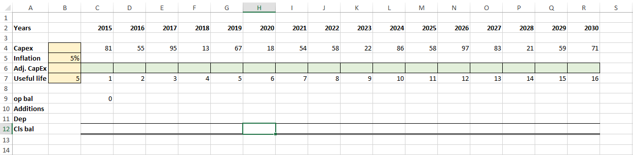
Step 1: Download the file and open it. You will see preliminary information already available arranged in row format. It looks like this:
Step 2: First we need inflation multiplier so that we can calculate adjusted CAPEX for each year. To calculate inflation multiplier the formula is:
(1+r)^n
where r is rate of interest and n is the number of years. So the base year will be n = 0 and with every next year “n” will increase by 1. To do the calculations in Excel we can use the formula.
Go to cell C5 and put this formula:
=(1+$B$5)^(COLUMN()-3)
Drag the fill handle to cell R5.
B4 contains the percentage value and COLUMN() function help increase the value as we drag the fill handle. “-3” is appended at the end as we are starting from column 3 therefore to make the resultant equal to 0, a weight is added.
In cell C6 put this formula and drag the fill handle to R5: =C4*C5
Step 3: We assume the opening balance of fixed asset is zero, so enter 0 in cell C9. Row 10 is about additions (acquisition of fixed assets). It will be adjusted capital expenditure figures. Therefore, in cell C10 put the formula: =C6 and drag the fill handle to R9.
Step 4: If we have the depreciation figures, we can calculate the closing balance by adding opening balance and additions during the year and deducting the depreciation of the year amount. To calculate the closing balance put the following formula in cell C12 and drag the fill handle to cell R12:
=C9+C10-C11
Step 4: To calculate the depreciation go to cell C10 and put the following formula:
=(SUMPRODUCT($C$6:$R$6,--($C$7:$R$7<=(COLUMN()-2)))-IF(C7>$B$7,SUMPRODUCT($C$6:$R$6,--($C$7:$R$7<=(COLUMN()-($B$7+2))))))/$B$7
This formula might look daunting and before we dissect it, lets understand the situation the easy way. Remember we are using straight line basis for depreciation and useful life is 5 years for each asset. Therefore, every 5 years the oldest asset will complete useful life and will be disposed off, if we make the schedule for each asset over the years with total of assets and depreciation each year, it will look like this:
Use scroll bar to go through the whole data. To the right you can see the sum for each year and the depreciation calculation as well. This is exactly we have done in the formula above but it has saved us all of this work! Amazing isn’t it 🙂
Though I recommend everyone to go through an easier tutorial on SUMPRODUCT to understand how it works and also the use of “double dash” by reading: Conditional SUM in Excel with SUMPRODUCT function.
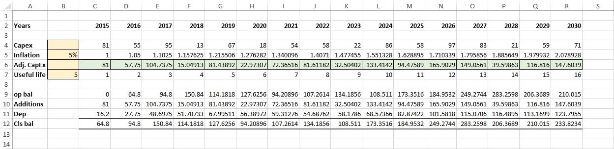
So once we have the depreciation calculation in place we have the forecast complete. And as formulas are based on cell values (for inflation, useful years) you can easily change them and model will update instantly.
The completed file looks like this:
You can download the fully worked file to play and learn. Enjoy!
Dear Mr. Fazal,
There is an assumption for depreciation, can you guide on it.
Capital Expenditure Assumptions
Asset Salvage Value (% of Capital Addition) 15%
Asset Useful Life 10 Years
Regards
The formula for the inflation rate above says (1+$B$4) should be $B$5.
Thanks for pointing out. Its corrected
The depreciation forecast working is excellent.
Thanks Saleem and welcome to PakAccountants!