A classical scenario to understand the excellence of Excel. There might be situations where we would like to split the email address in two parts i.e. the username (part at the left of @ symbol) and the domain name (part at the right of @ symbol).
For example [email protected] has the username hasaanfazalpk and gmail.com is the domain name. So consider a situation that you have thousands of such email addresses and you want to extract the username and domain name of each. This is where Excel shines again.
Method 1: Using Text to column tool
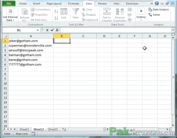
Step 1: Select the range from which you would like to extract or separate usernames/domain names
Step 2: Click Data tab in the Excel ribbon and hit text to column button in Data tools group
Step 3: Make sure the delimited option is selected and hit Next button
Step 4: Make sure only Other box is checked under delimiters options and in the box punch in @ symbol and hit Next button
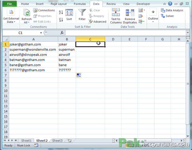
Step 5: In the last step select the cell where you would like Excel to produce the results. In our example it is: $B$2. Hit Finish button.
It is the simplest possible method to get this sort of job done and it is pretty fast too.
Following animation walks you through the whole process:

Method 2: Using Excel functions
We can get this job done using Excel functions as well and there are lots of different ways in which we can devise a formula to get it done. The difference in this technique beside the use of formula is that you have select the range where you want the output in the start of the process as oppose to the Method 1 where we selected it as the last step.
The other notable difference is the Text to Column is more of a split approach whereas using formula it is more of an extract approach. In simple words TtC splits the email address in two in one stroke whereas with formulas we extract a specific portion.
Extracting Username
Step 1: With the email addresses in column A, to extract username type this formula in cell B1 and hit Enter key:
=LEFT(A1,FIND("@",A1)-1)
Following animation shows the result of this formaula:
Understanding LEFT
LEFT function help us extract the specified number of characters from the text string starting from the left.
LEFT function has the following syntax:
LEFT(text, [num_chars])
where;
text: can either be the text you mention or the cell address that contains the text.
num_chars: number of characters you want LEFT function to pull out starting from the left. So in this argument you have to mention a number.
For example:
=LEFT(“Hasaan”,3) will print Has as a result.
Talking about email address we can have the username portion of email address of varying length, therefore we cannot specify a single number to extract the username from email address. Lets understand it with an example:
[email protected] this email address has 13 characters long username
[email protected] this email address has 11 characters long username
In short, using LEFT function with a hard coded number is not the solution for us. But we do know that username and domain name have a “divider” between then in the form of @ symbol. And if by any chance we can find out the position @ symbol in the email address, we can get LEFT function working for us. This is where Excel’s FIND function help us.
Understanding FIND
FIND function helps us find the location of specified text within specified text string in the form of a number.
FIND function has the following syntax:
FIND(find_text, within_text, [start_num])
where:
find_text: is what you like to find
within_text: is where you want to find
[start_num]: is where you want excel to start from i.e. excel will simply jump this many number of characters from the left of text string mentioned in within_text argument. It is an optional argument and if left blank excel will start finding from the first character.
For example:
=FIND(“s”,”Hasaan”) will result in 3 where 3 is the location of S in the specified text string Hasaan
With the function of each function understood, now we can combine them for our good 🙂
Have a look at the formula I mentioned above again:
=LEFT(A1,FIND(“@”,A1)-1)
As the FIND function is inside most function, Excel will start with solving it first (just like mathematics). FIND function will look for @ symbol in the text mention in cell A1. The address is [email protected]. Here the @ symbol is residing at 6th position. And this is the number that will fed to LEFT function and it will extract the first 6 characters starting from left from the text string mentioned in cell A1.
But here is the catch if we count the first 6 characters in [email protected] this will include the symbol as well which we don’t want. And to solve we simple have to reduce the result by one character. And that is the reason we have “-1” in FIND(“@”,A1)-1 part of the formula.
Extracting Domain name
Now that we have understood how to get the username, it will be easy for us to understand the mechanics for extracting domain name.
With cell A1 being the one with the email address in cell C1 put this formula to extract the domain name:
=RIGHT(A1,LEN(A1)-FIND(“@”,A1))
Hit Enter key on the keyboard and drag the fill handle to get the domain names from other email addresses to in the range.
Here is the illustration for you to see it in action:
The above formula has two main changes:
- Instead of LEFT now are using RIGHT function so that Excel start counting from the right of text string.
- LEN is the additional function which counts the total number of characters in the text string.
Now I will leave you to your common sense and a hint of imagination to get your neurons working to understand how the formula works 🙂
Hi everyone,
plz help if in the same function I want to make first letter big for user name.
this is very urgent plz help
nice very good news ,thanks
Hi,
I have 2 mail ID’s in a cell and want domain name from any one mail id’s like below.
[email protected], [email protected]
need: romail.com
With 2 mail IDs in cell A1, one possible solution is this: =RIGHT(A1,FIND(“,”,A1)-FIND(“@”,A1)-1)
Not working
Hey Ashish thank you for reaching. Can you elaborate what is not working?