OFFSET
Determines a range of cells with specific number of rows and columns after displacing certain number of rows and columns from the given reference
Determines a range of cells with specific number of rows and columns after displacing certain number of rows and columns from the given reference
Syntax of Excel OFFSET formula:
=OFFSET(reference, rows, cols, [height], [width])
In words:
=Determine the range by offsetting(from this reference, coming up/down this number of rows, going left/right this many columns, [of this height], [and this width])
Explanation
OFFSET functions help makes the calculation dynamic by making the lookup range to be dynamic as you can move it up, down, left or right. Lets understand how this works.
Consider the following data:
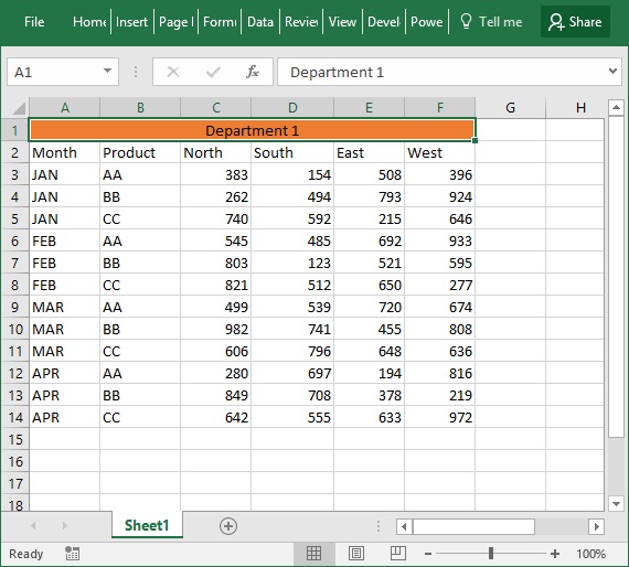
If you have Department 1 selected then it is cell A1. If cells are merged, then cell address is of the top left most cell.
If you want to get the sales value for Product CC for the month of JAN in East region, your formula will be like this:
=OFFSET(A1,4,4,1,1) and it will return 215 which is the sales value of East region of product CC for the month of JAN. So what really happened?
You asked Excel to offset or simply displace starting from cell A1 and move 4 rows under reaching cell A5, once here move 4 columns to the right thus reaching cell E5 and fetch reference which is 1 row high and 1 column wide thus returning the value in cell E5.
Get the value
This one is discussed in the explanation above
Get the range of cells
Lets say we want to sum the sales of product CC for the month of JAN for all regions for this the formula will be:
=SUM(OFFSET(A1,4,2,1,4))
Sum the sales of all products of latest month
Lets say we want to sum the sales of all products in a particular region e.g. North whatever the latest month so that every time data is updated we don’t have to change the formula, then after converting the range to table we can use the following formula:
=SUM(OFFSET(A1,COUNTA(Table1[North])-1,2,3,1))